Compute and plot all contrasts and test results from a linear model by automating the use of emmeans tables and plots.
Source:R/e_plot_model_contrasts.R
e_plot_model_contrasts.RdVariable labels can be provided by labelling your data with the labelled::var_label() command.
e_plot_model_contrasts(
  fit = NULL,
  dat_cont = NULL,
  choose_contrasts = NULL,
  sw_table_in_plot = TRUE,
  sw_points_in_plot = TRUE,
  sw_ribbon_in_plot = TRUE,
  adjust_method = c("none", "tukey", "scheffe", "sidak", "bonferroni", "dunnettx",
    "mvt")[4],
  CI_level = 0.95,
  sw_glm_scale = c("link", "response")[2],
  sw_print = TRUE,
  sw_marginal_even_if_interaction = FALSE,
  sw_TWI_plots_keep = c("singles", "both", "all")[3],
  sw_TWI_both_orientation = c("wide", "tall")[1],
  sw_plot_quantiles_values = c("quantiles", "values")[1],
  plot_quantiles = c(0.05, 0.25, 0.5, 0.75, 0.95),
  sw_quantile_type = 7,
  plot_values = NULL,
  emmip_rg.limit = 10000
)
Arguments
- fit
(required) model object: lm, glm, lmerModLmerTest (from
lme4::lmer, or lmerMod (fromlmerTest::as_lmerModLmerTest)- dat_cont
(required) data used for the lm object (only used for variable labels using labelled::var_label()
- choose_contrasts
is a list of effects to plot, such as c("hp", "vs:wt"); NULL does all in model.
- sw_table_in_plot
T/F put table of results in caption of plot
- sw_points_in_plot
T/F include marginal points in numeric plot
- sw_ribbon_in_plot
T/F include error bands in numeric plot
- adjust_method
- CI_level
level from
?emmeans::emmeans- sw_glm_scale
for glm fit, choose results on the "link" or "response" (default) scale (e.g., for logistic regression, link is logit scale and response is probability scale)
- sw_print
T/F whether to print results as this function runs
- sw_marginal_even_if_interaction
T/F whether to also calculate marginal results when involved in interaction(s)
- sw_TWI_plots_keep
two-way interaction plots are plotted for each variable conditional on the other. Plots are created separately ("singles") or together in a grid ("both"), and "all" keeps the singles and the grid version.
- sw_TWI_both_orientation
"tall" or "wide" orientation for when both two-way interaction plots are combined in a grid
- sw_plot_quantiles_values
"quantiles" or "values" to specify whether to plot quantiles of the numeric variable or specified values
- plot_quantiles
quantiles plotted for numeric:numeric interaction plots, if
sw_plot_quantiles_valuesis "quantiles"- sw_quantile_type
quantile type as specified in
?stats::quantile.- plot_values
a named list for values plotted for a single specified numeric:numeric interaction plot, if
sw_plot_quantiles_valuesis "values". Specify a specific contrast, for example:choose_contrasts = "disp:hp". Then specify the values for each variable, for example:plot_values = list(hp = c(75, 100, 150, 200, 250), disp = c(80, 120, 200, 350, 450))- emmip_rg.limit
from emmeans package, increase from 10000 if "Error: The rows of your requested reference grid would be 10000, which exceeds the limit of XXXXX (not including any multivariate responses)."
Value
out a list of three lists: "plots", "tables" , and "text", each have results for each contrast that was computed. "plots" is a list of ggplot objects to plot separately or arrange in a grid. "tables" is a list of emmeans tables to print. "text" is the caption text for the plots.
Details
Plot interpretation: This EMM plot (Estimated Marginal Means, aka Least-Squares Means) is only available when conditioning on one variable. The blue bars are confidence intervals for the EMMs; don't ever use confidence intervals for EMMs to perform comparisons --- they can be very misleading. The red arrows are for the comparisons between means; the degree to which the "comparison arrows" overlap reflects as much as possible the significance of the comparison of the two estimates. If an arrow from one mean overlaps an arrow from another group, the difference is not significant, based on the adjust setting (which defaults to "tukey").
Examples
# Data for testing
dat_cont <-
dat_mtcars_e
# Set specific model with some interactions
form_model <-
mpg ~ cyl + disp + hp + wt + vs + am + cyl:vs + disp:hp + hp:vs
fit <-
lm(
formula = form_model
, data = dat_cont
)
car::Anova(fit) #, type = 3)
#> Note: model has aliased coefficients
#> sums of squares computed by model comparison
#> Anova Table (Type II tests)
#>
#> Response: mpg
#> Sum Sq Df F value Pr(>F)
#> cyl 0.955 2 0.0818 0.92176
#> disp 0.349 1 0.0598 0.80923
#> hp 36.912 1 6.3201 0.02016 *
#> wt 31.610 1 5.4123 0.03009 *
#> vs 1.889 1 0.3235 0.57556
#> am 3.593 1 0.6152 0.44159
#> cyl:vs 1.746 1 0.2989 0.59032
#> disp:hp 1.930 1 0.3305 0.57150
#> hp:vs 5.004 1 0.8568 0.36515
#> Residuals 122.648 21
#> ---
#> Signif. codes: 0 '***' 0.001 '**' 0.01 '*' 0.05 '.' 0.1 ' ' 1
summary(fit)
#>
#> Call:
#> lm(formula = form_model, data = dat_cont)
#>
#> Residuals:
#> Min 1Q Median 3Q Max
#> -3.2634 -1.6094 -0.3633 1.3947 3.8193
#>
#> Coefficients: (1 not defined because of singularities)
#> Estimate Std. Error t value Pr(>|t|)
#> (Intercept) 3.598e+01 8.628e+00 4.170 0.000433 ***
#> cylsix -1.967e+00 3.313e+00 -0.594 0.559012
#> cyleight -8.898e-01 4.369e+00 -0.204 0.840561
#> disp -1.501e-02 3.403e-02 -0.441 0.663566
#> hp -5.193e-02 5.031e-02 -1.032 0.313707
#> wt -2.821e+00 1.213e+00 -2.326 0.030086 *
#> vsstraight 5.149e+00 5.521e+00 0.933 0.361603
#> ammanual 1.521e+00 1.939e+00 0.784 0.441592
#> cylsix:vsstraight 1.970e+00 3.603e+00 0.547 0.590322
#> cyleight:vsstraight NA NA NA NA
#> disp:hp 9.752e-05 1.696e-04 0.575 0.571500
#> hp:vsstraight -4.915e-02 5.310e-02 -0.926 0.365152
#> ---
#> Signif. codes: 0 '***' 0.001 '**' 0.01 '*' 0.05 '.' 0.1 ' ' 1
#>
#> Residual standard error: 2.417 on 21 degrees of freedom
#> Multiple R-squared: 0.8911, Adjusted R-squared: 0.8392
#> F-statistic: 17.18 on 10 and 21 DF, p-value: 5.984e-08
#>
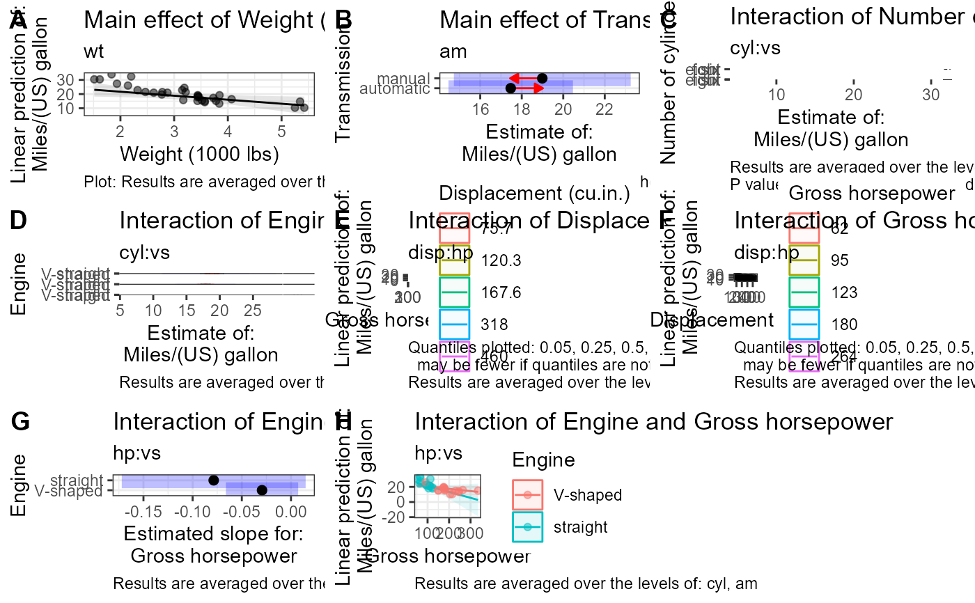
# all contrasts from model
fit_contrasts <-
e_plot_model_contrasts(
fit = fit
, dat_cont = dat_cont
, sw_print = FALSE
, sw_table_in_plot = FALSE
, sw_TWI_plots_keep = "singles"
, sw_quantile_type = 1
)
#> e_plot_model_contrasts: Skipping "cyl" since involved in interactions.
#> e_plot_model_contrasts: Skipping "disp" since involved in interactions.
#> e_plot_model_contrasts: Skipping "hp" since involved in interactions.
#> e_plot_model_contrasts: Skipping "vs" since involved in interactions.
#> Warning: Comparison discrepancy in group "straight", four - six:
#> Target overlap = 0.9995, overlap on graph = -101.2269
#> Warning: Comparison discrepancy in group "straight", four - six:
#> Target overlap = 0.9995, overlap on graph = -104.1881
fit_contrasts$tables # to print tables
#> $wt
#> $wt$est
#> wt wt.trend SE df lower.CL upper.CL
#> 3.22 -2.82 1.21 21 -5.34 -0.299
#>
#> Results are averaged over the levels of: cyl, vs, am
#> Confidence level used: 0.95
#>
#>
#> $am
#> $am$est
#> am emmean SE df lower.CL upper.CL
#> automatic 17.5 1.25 21 14.5 20.5
#> manual 19.0 1.77 21 14.7 23.3
#>
#> Results are averaged over the levels of: cyl, vs
#> Confidence level used: 0.95
#> Conf-level adjustment: sidak method for 2 estimates
#>
#> $am$cont
#> contrast estimate SE df t.ratio p.value
#> automatic - manual -1.52 1.94 21 -0.784 0.4416
#>
#> Results are averaged over the levels of: cyl, vs
#>
#>
#> $`cyl:vs`
#> $`cyl:vs`$est
#> cyl = four:
#> vs emmean SE df lower.CL upper.CL
#> V-shaped 19.9 3.53 21 11.39 28.4
#> straight 17.8 2.73 21 11.24 24.4
#>
#> cyl = six:
#> vs emmean SE df lower.CL upper.CL
#> V-shaped 17.9 1.82 21 13.54 22.3
#> straight 17.8 1.91 21 13.23 22.4
#>
#> cyl = eight:
#> vs emmean SE df lower.CL upper.CL
#> V-shaped 19.0 1.67 21 14.96 23.0
#> straight 16.9 4.54 21 6.01 27.9
#>
#> Results are averaged over the levels of: am
#> Confidence level used: 0.95
#> Conf-level adjustment: sidak method for 2 estimates
#>
#> $`cyl:vs`$cont
#> cyl = four:
#> contrast estimate SE df t.ratio p.value
#> (V-shaped) - straight 2.0601 3.97 21 0.519 0.6095
#>
#> cyl = six:
#> contrast estimate SE df t.ratio p.value
#> (V-shaped) - straight 0.0901 2.82 21 0.032 0.9748
#>
#> cyl = eight:
#> contrast estimate SE df t.ratio p.value
#> (V-shaped) - straight nonEst NA NA NA NA
#>
#> Results are averaged over the levels of: am
#>
#>
#> $`hp:vs`
#> $`hp:vs`$est
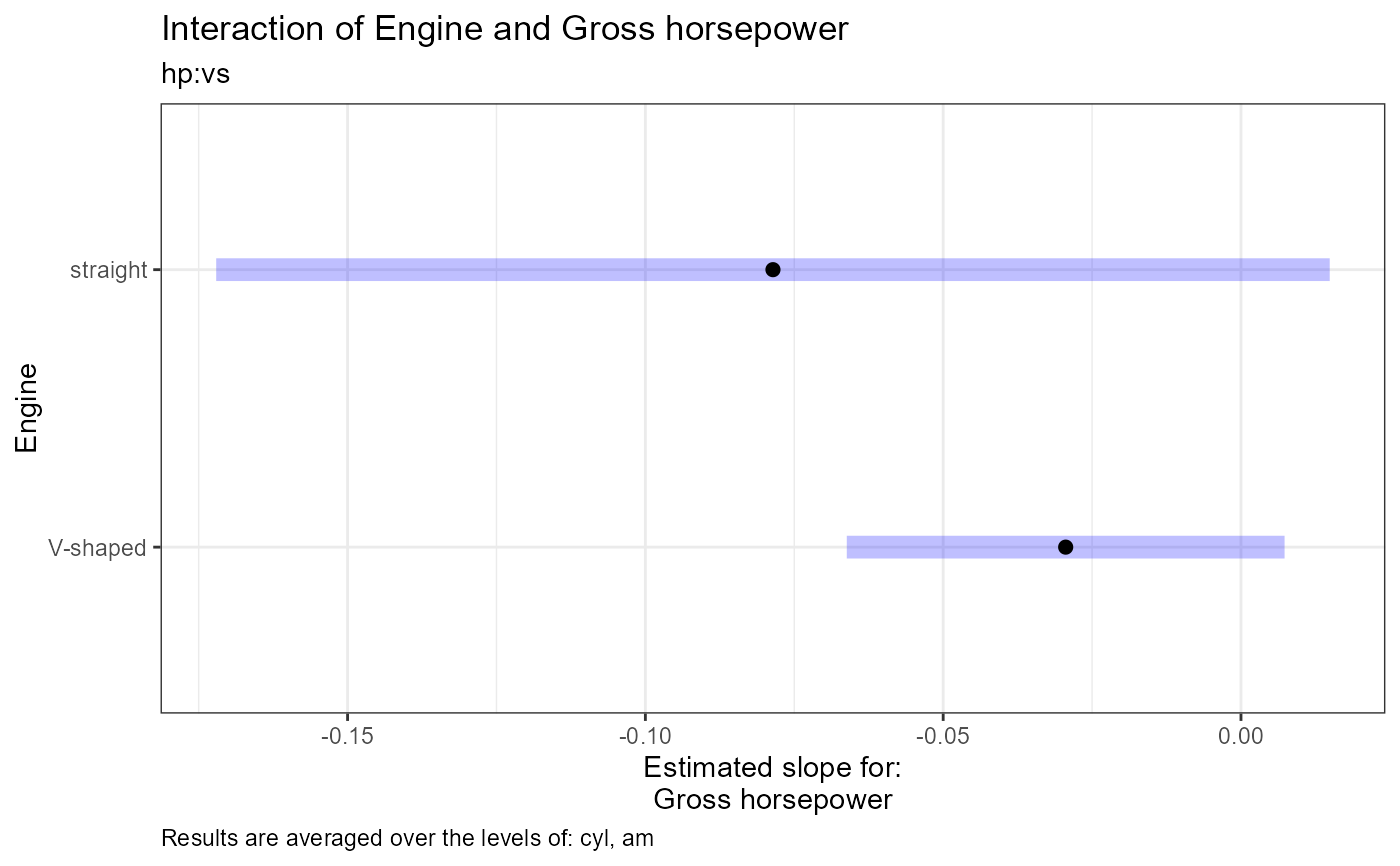
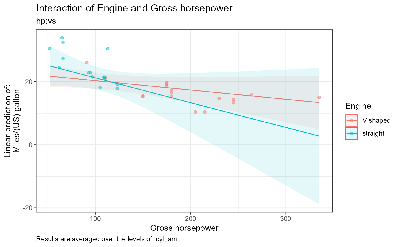
#> vs hp.trend SE df lower.CL upper.CL
#> V-shaped -0.0294 0.0177 21 -0.0662 0.00732
#> straight -0.0786 0.0449 21 -0.1721 0.01490
#>
#> Results are averaged over the levels of: cyl, am
#> Confidence level used: 0.95
#>
#> $`hp:vs`$cont
#> contrast estimate SE df t.ratio p.value
#> (V-shaped) - straight 0.0491 0.0531 21 0.926 0.3652
#>
#> Results are averaged over the levels of: cyl, am
#>
#>
fit_contrasts$plots # to print plots
#> $wt
 #>
#> $am
#>
#> $am
 #>
#> $`cyl:vs`
#> $`cyl:vs`[[1]]
#>
#> $`cyl:vs`
#> $`cyl:vs`[[1]]
 #>
#> $`cyl:vs`[[2]]
#>
#> $`cyl:vs`[[2]]
 #>
#>
#> $`disp:hp`
#> $`disp:hp`[[1]]
#>
#>
#> $`disp:hp`
#> $`disp:hp`[[1]]
 #>
#> $`disp:hp`[[2]]
#>
#> $`disp:hp`[[2]]
 #>
#>
#> $`hp:vs`
#> $`hp:vs`[[1]]
#>
#>
#> $`hp:vs`
#> $`hp:vs`[[1]]
 #>
#> $`hp:vs`[[2]]
#>
#> $`hp:vs`[[2]]
 #>
#>
fit_contrasts$text # to print caption text
#> $wt
#> $wt[[1]]
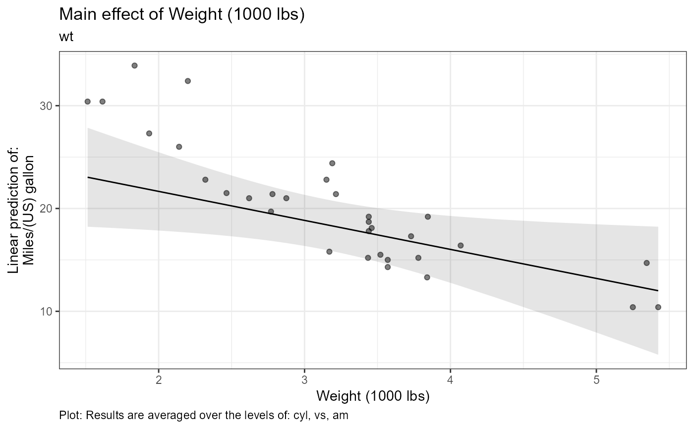
#> [1] "Estimate (n = 32): (at mean = 3.22): -2.82, 95% CI: (-5.34, -0.299)"
#> [2] "Tables: Results are averaged over the levels of: cyl, vs, am"
#> [3] "Plot: Results are averaged over the levels of: cyl, vs, am"
#>
#> $wt[[2]]
#> [1] "Estimate (n = 32): (at mean = 3.22): -2.82, 95% CI: (-5.34, -0.299)"
#> [2] "Tables: Confidence level used: 0.95"
#> [3] "Plot: Confidence level used: 0.95"
#>
#>
#> $am
#> $am[[1]]
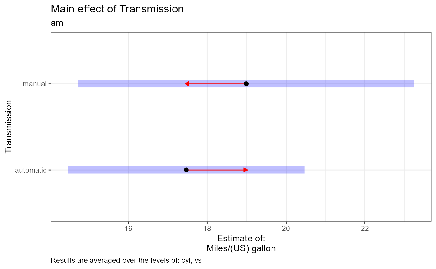
#> [1] "Estimate (n = 19): automatic = 17.5, 95% CI: (14.5, 20.5)"
#> [2] "Estimate (n = 13): manual = 19, 95% CI: (14.7, 23.3)"
#> [3] "Contrast: automatic - manual = -1.52, p-value = 0.4416"
#> [4] "Results are averaged over the levels of: cyl, vs"
#>
#>
#> $`cyl:vs`
#> $`cyl:vs`[[1]]
#> $`cyl:vs`[[1]][[1]]
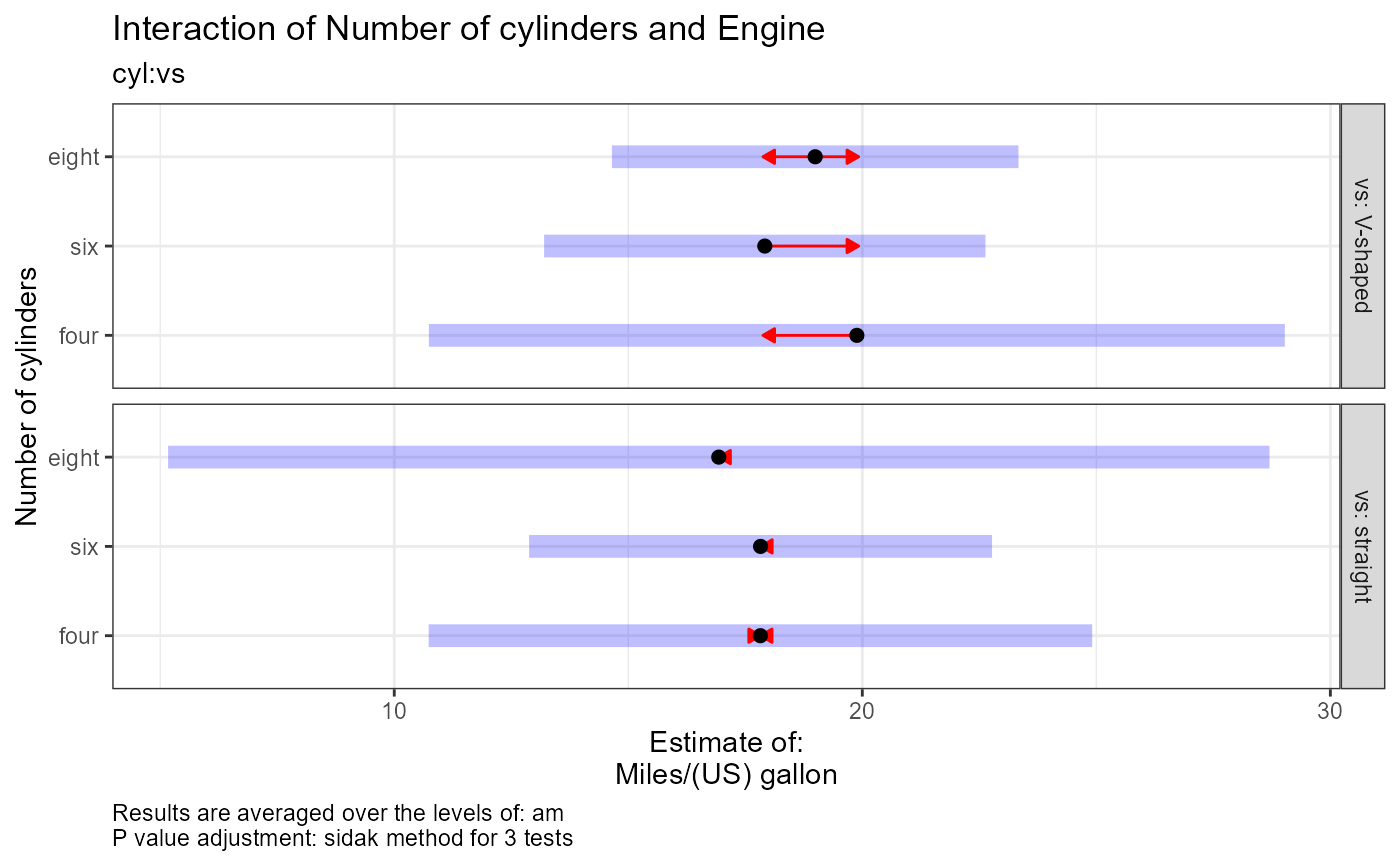
#> [1] "vs = V-shaped:"
#> [2] "Estimate (n = 1): four = 19.9, 95% CI: (10.7, 29)"
#> [3] "Estimate (n = 3): six = 17.9, 95% CI: (13.2, 22.6)"
#> [4] "Estimate (n = 14): eight = 19, 95% CI: (14.7, 23.3)"
#> [5] "vs = straight:"
#> [6] "Estimate (n = 10): four = 17.8, 95% CI: (10.7, 24.9)"
#> [7] "Estimate (n = 4): six = 17.8, 95% CI: (12.9, 22.8)"
#> [8] "Estimate (n = 0): eight = 16.9, 95% CI: (5.17, 28.7)"
#> [9] ""
#> [10] "vs = V-shaped:"
#> [11] "Contrast: four - six = 1.97, p-value = 0.9142"
#> [12] "Contrast: four - eight = 0.89, p-value = 0.9959"
#> [13] "Contrast: six - eight = -1.08, p-value = 0.9789"
#> [14] "vs = straight:"
#> [15] "Contrast: four - six = -0.00314, p-value = 1"
#> [16] "Contrast: four - eight = NA, p-value = NA"
#> [17] "Contrast: six - eight = NA, p-value = NA"
#> [18] ""
#> [19] "Results are averaged over the levels of: am"
#> [20] "P value adjustment: sidak method for 3 tests"
#>
#>
#> $`cyl:vs`[[2]]
#> $`cyl:vs`[[2]][[1]]
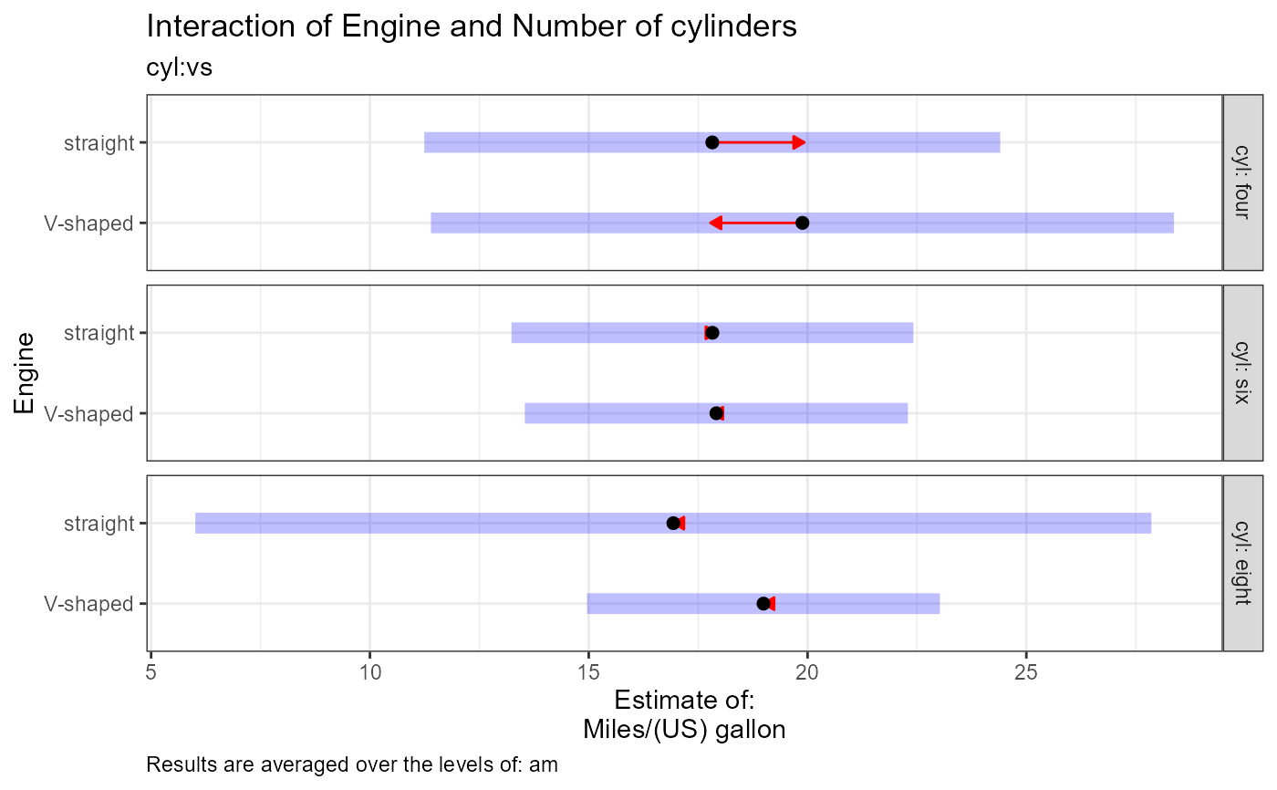
#> [1] "cyl = four:"
#> [2] "Estimate (n = 1): V-shaped = 19.9, 95% CI: (11.4, 28.4)"
#> [3] "Estimate (n = 10): straight = 17.8, 95% CI: (11.2, 24.4)"
#> [4] "cyl = six:"
#> [5] "Estimate (n = 3): V-shaped = 17.9, 95% CI: (13.5, 22.3)"
#> [6] "Estimate (n = 4): straight = 17.8, 95% CI: (13.2, 22.4)"
#> [7] "cyl = eight:"
#> [8] "Estimate (n = 14): V-shaped = 19, 95% CI: (15, 23)"
#> [9] "Estimate (n = 0): straight = 16.9, 95% CI: (6.01, 27.9)"
#> [10] ""
#> [11] "cyl = four:"
#> [12] "Contrast: (V-shaped) - straight = 2.06, p-value = 0.6095"
#> [13] "cyl = six:"
#> [14] "Contrast: (V-shaped) - straight = 0.0901, p-value = 0.9748"
#> [15] "cyl = eight:"
#> [16] "Contrast: (V-shaped) - straight = NA, p-value = NA"
#> [17] ""
#> [18] "Results are averaged over the levels of: am"
#>
#>
#>
#> $`disp:hp`
#> $`disp:hp`[[1]]
#> $`disp:hp`[[1]][[1]]
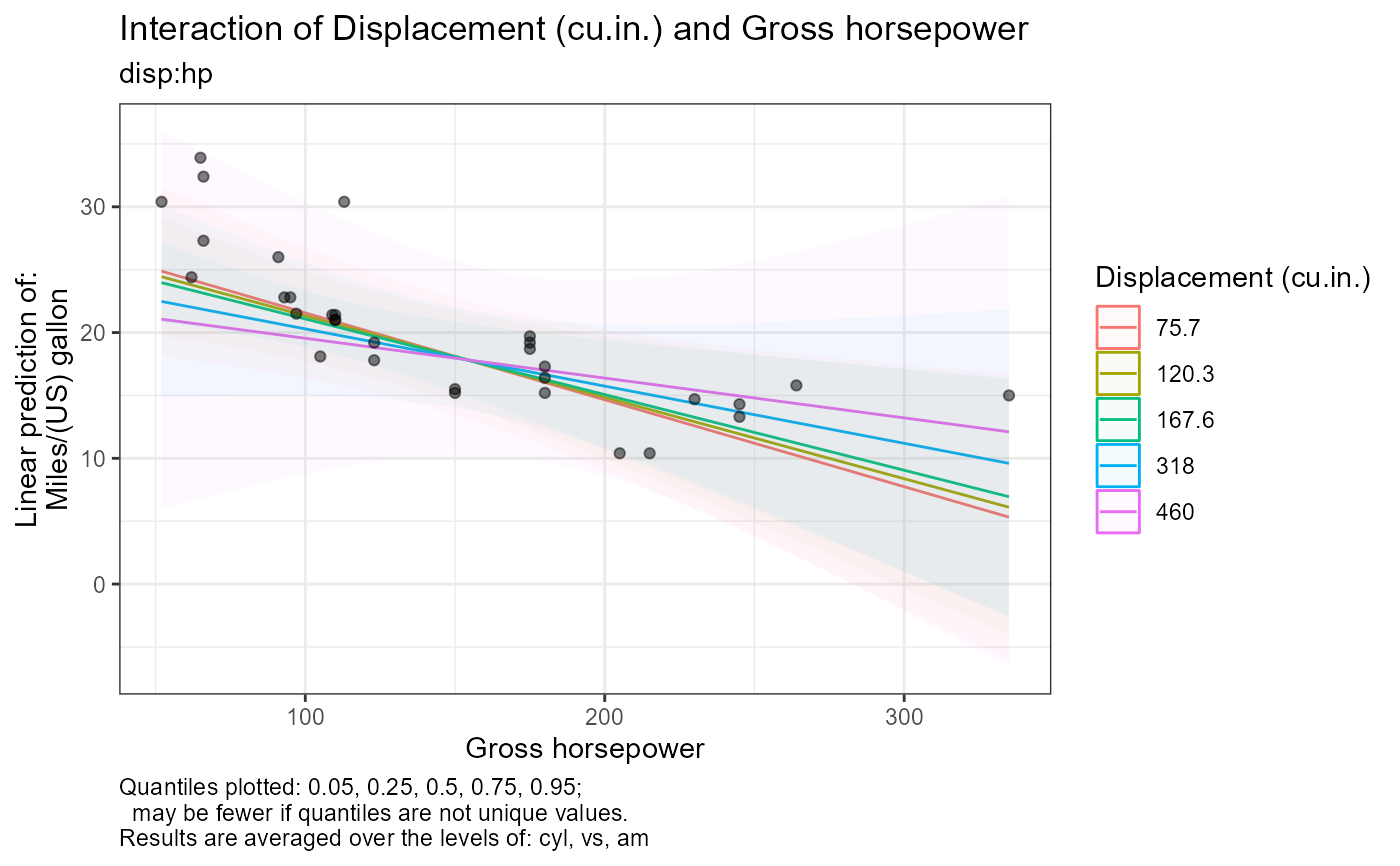
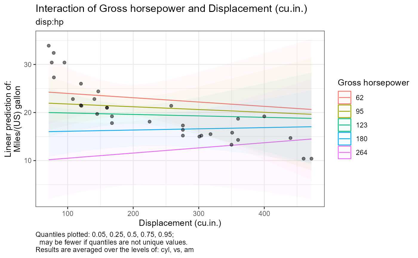
#> [1] "Quantiles plotted: 0.05, 0.25, 0.5, 0.75, 0.95;"
#> [2] " may be fewer if quantiles are not unique values."
#> [3] "Results are averaged over the levels of: cyl, vs, am"
#>
#> $`disp:hp`[[1]][[2]]
#> [1] "Quantiles plotted: 0.05, 0.25, 0.5, 0.75, 0.95;"
#> [2] " may be fewer if quantiles are not unique values."
#> [3] "Confidence level used: 0.95"
#>
#>
#> $`disp:hp`[[2]]
#> $`disp:hp`[[2]][[1]]
#> [1] "Quantiles plotted: 0.05, 0.25, 0.5, 0.75, 0.95;"
#> [2] " may be fewer if quantiles are not unique values."
#> [3] "Results are averaged over the levels of: cyl, vs, am"
#>
#> $`disp:hp`[[2]][[2]]
#> [1] "Quantiles plotted: 0.05, 0.25, 0.5, 0.75, 0.95;"
#> [2] " may be fewer if quantiles are not unique values."
#> [3] "Confidence level used: 0.95"
#>
#>
#>
#> $`hp:vs`
#> $`hp:vs`[[1]]
#> $`hp:vs`[[1]][[1]]
#> [1] "Estimate (n = 18): V-shaped = -0.0294, 95% CI: (-0.0662, 0.00732)"
#> [2] "Estimate (n = 14): straight = -0.0786, 95% CI: (-0.172, 0.0149)"
#> [3] "Contrast: (V-shaped) - straight = 0.0491, p-value = 0.3652"
#> [4] "Results are averaged over the levels of: cyl, am"
#>
#>
#> $`hp:vs`[[2]]
#> $`hp:vs`[[2]][[1]]
#> [1] "Estimate (n = 18): V-shaped = -0.0294, 95% CI: (-0.0662, 0.00732)"
#> [2] "Estimate (n = 14): straight = -0.0786, 95% CI: (-0.172, 0.0149)"
#> [3] "Contrast: (V-shaped) - straight = 0.0491, p-value = 0.3652"
#> [4] "Results are averaged over the levels of: cyl, am"
#>
#>
#>
## To plot all contrasts in a plot grid:
# Since plot interactions have sublists of plots, we want to pull those out
# into a one-level plot list.
# The code here works for sw_TWI_plots_keep = "singles"
# which will make each plot the same size in the plot_grid() below.
# For a publications, you'll want to manually choose which plots to show.
# index for plot list,
# needed since interactions add 2 plots to the list, so the number of terms
# is not necessarily the same as the number of plots.
i_list <- 0
# initialize a list of plots
p_list <- list()
for (i_term in 1:length(fit_contrasts$plots)) {
## i_term = 1
# extract the name of the plot
n_list <- names(fit_contrasts$plots)[i_term]
# test whether the name has a colon ":"; if so, it's an interaction
if (stringr::str_detect(string = n_list, pattern = stringr::fixed(":"))) {
# an two-way interaction has two plots
# first plot
i_list <- i_list + 1
p_list[[ i_list ]] <- fit_contrasts$plots[[ i_term ]][[ 1 ]]
# second plot
i_list <- i_list + 1
p_list[[ i_list ]] <- fit_contrasts$plots[[ i_term ]][[ 2 ]]
} else {
# not an interaction, only one plot
i_list <- i_list + 1
p_list[[ i_list ]] <- fit_contrasts$plots[[ i_term ]]
} # if
} # for
p_arranged <-
cowplot::plot_grid(
plotlist = p_list
, nrow = NULL
, ncol = 3
, labels = "AUTO"
)
p_arranged %>% print()
#>
#>
fit_contrasts$text # to print caption text
#> $wt
#> $wt[[1]]
#> [1] "Estimate (n = 32): (at mean = 3.22): -2.82, 95% CI: (-5.34, -0.299)"
#> [2] "Tables: Results are averaged over the levels of: cyl, vs, am"
#> [3] "Plot: Results are averaged over the levels of: cyl, vs, am"
#>
#> $wt[[2]]
#> [1] "Estimate (n = 32): (at mean = 3.22): -2.82, 95% CI: (-5.34, -0.299)"
#> [2] "Tables: Confidence level used: 0.95"
#> [3] "Plot: Confidence level used: 0.95"
#>
#>
#> $am
#> $am[[1]]
#> [1] "Estimate (n = 19): automatic = 17.5, 95% CI: (14.5, 20.5)"
#> [2] "Estimate (n = 13): manual = 19, 95% CI: (14.7, 23.3)"
#> [3] "Contrast: automatic - manual = -1.52, p-value = 0.4416"
#> [4] "Results are averaged over the levels of: cyl, vs"
#>
#>
#> $`cyl:vs`
#> $`cyl:vs`[[1]]
#> $`cyl:vs`[[1]][[1]]
#> [1] "vs = V-shaped:"
#> [2] "Estimate (n = 1): four = 19.9, 95% CI: (10.7, 29)"
#> [3] "Estimate (n = 3): six = 17.9, 95% CI: (13.2, 22.6)"
#> [4] "Estimate (n = 14): eight = 19, 95% CI: (14.7, 23.3)"
#> [5] "vs = straight:"
#> [6] "Estimate (n = 10): four = 17.8, 95% CI: (10.7, 24.9)"
#> [7] "Estimate (n = 4): six = 17.8, 95% CI: (12.9, 22.8)"
#> [8] "Estimate (n = 0): eight = 16.9, 95% CI: (5.17, 28.7)"
#> [9] ""
#> [10] "vs = V-shaped:"
#> [11] "Contrast: four - six = 1.97, p-value = 0.9142"
#> [12] "Contrast: four - eight = 0.89, p-value = 0.9959"
#> [13] "Contrast: six - eight = -1.08, p-value = 0.9789"
#> [14] "vs = straight:"
#> [15] "Contrast: four - six = -0.00314, p-value = 1"
#> [16] "Contrast: four - eight = NA, p-value = NA"
#> [17] "Contrast: six - eight = NA, p-value = NA"
#> [18] ""
#> [19] "Results are averaged over the levels of: am"
#> [20] "P value adjustment: sidak method for 3 tests"
#>
#>
#> $`cyl:vs`[[2]]
#> $`cyl:vs`[[2]][[1]]
#> [1] "cyl = four:"
#> [2] "Estimate (n = 1): V-shaped = 19.9, 95% CI: (11.4, 28.4)"
#> [3] "Estimate (n = 10): straight = 17.8, 95% CI: (11.2, 24.4)"
#> [4] "cyl = six:"
#> [5] "Estimate (n = 3): V-shaped = 17.9, 95% CI: (13.5, 22.3)"
#> [6] "Estimate (n = 4): straight = 17.8, 95% CI: (13.2, 22.4)"
#> [7] "cyl = eight:"
#> [8] "Estimate (n = 14): V-shaped = 19, 95% CI: (15, 23)"
#> [9] "Estimate (n = 0): straight = 16.9, 95% CI: (6.01, 27.9)"
#> [10] ""
#> [11] "cyl = four:"
#> [12] "Contrast: (V-shaped) - straight = 2.06, p-value = 0.6095"
#> [13] "cyl = six:"
#> [14] "Contrast: (V-shaped) - straight = 0.0901, p-value = 0.9748"
#> [15] "cyl = eight:"
#> [16] "Contrast: (V-shaped) - straight = NA, p-value = NA"
#> [17] ""
#> [18] "Results are averaged over the levels of: am"
#>
#>
#>
#> $`disp:hp`
#> $`disp:hp`[[1]]
#> $`disp:hp`[[1]][[1]]
#> [1] "Quantiles plotted: 0.05, 0.25, 0.5, 0.75, 0.95;"
#> [2] " may be fewer if quantiles are not unique values."
#> [3] "Results are averaged over the levels of: cyl, vs, am"
#>
#> $`disp:hp`[[1]][[2]]
#> [1] "Quantiles plotted: 0.05, 0.25, 0.5, 0.75, 0.95;"
#> [2] " may be fewer if quantiles are not unique values."
#> [3] "Confidence level used: 0.95"
#>
#>
#> $`disp:hp`[[2]]
#> $`disp:hp`[[2]][[1]]
#> [1] "Quantiles plotted: 0.05, 0.25, 0.5, 0.75, 0.95;"
#> [2] " may be fewer if quantiles are not unique values."
#> [3] "Results are averaged over the levels of: cyl, vs, am"
#>
#> $`disp:hp`[[2]][[2]]
#> [1] "Quantiles plotted: 0.05, 0.25, 0.5, 0.75, 0.95;"
#> [2] " may be fewer if quantiles are not unique values."
#> [3] "Confidence level used: 0.95"
#>
#>
#>
#> $`hp:vs`
#> $`hp:vs`[[1]]
#> $`hp:vs`[[1]][[1]]
#> [1] "Estimate (n = 18): V-shaped = -0.0294, 95% CI: (-0.0662, 0.00732)"
#> [2] "Estimate (n = 14): straight = -0.0786, 95% CI: (-0.172, 0.0149)"
#> [3] "Contrast: (V-shaped) - straight = 0.0491, p-value = 0.3652"
#> [4] "Results are averaged over the levels of: cyl, am"
#>
#>
#> $`hp:vs`[[2]]
#> $`hp:vs`[[2]][[1]]
#> [1] "Estimate (n = 18): V-shaped = -0.0294, 95% CI: (-0.0662, 0.00732)"
#> [2] "Estimate (n = 14): straight = -0.0786, 95% CI: (-0.172, 0.0149)"
#> [3] "Contrast: (V-shaped) - straight = 0.0491, p-value = 0.3652"
#> [4] "Results are averaged over the levels of: cyl, am"
#>
#>
#>
## To plot all contrasts in a plot grid:
# Since plot interactions have sublists of plots, we want to pull those out
# into a one-level plot list.
# The code here works for sw_TWI_plots_keep = "singles"
# which will make each plot the same size in the plot_grid() below.
# For a publications, you'll want to manually choose which plots to show.
# index for plot list,
# needed since interactions add 2 plots to the list, so the number of terms
# is not necessarily the same as the number of plots.
i_list <- 0
# initialize a list of plots
p_list <- list()
for (i_term in 1:length(fit_contrasts$plots)) {
## i_term = 1
# extract the name of the plot
n_list <- names(fit_contrasts$plots)[i_term]
# test whether the name has a colon ":"; if so, it's an interaction
if (stringr::str_detect(string = n_list, pattern = stringr::fixed(":"))) {
# an two-way interaction has two plots
# first plot
i_list <- i_list + 1
p_list[[ i_list ]] <- fit_contrasts$plots[[ i_term ]][[ 1 ]]
# second plot
i_list <- i_list + 1
p_list[[ i_list ]] <- fit_contrasts$plots[[ i_term ]][[ 2 ]]
} else {
# not an interaction, only one plot
i_list <- i_list + 1
p_list[[ i_list ]] <- fit_contrasts$plots[[ i_term ]]
} # if
} # for
p_arranged <-
cowplot::plot_grid(
plotlist = p_list
, nrow = NULL
, ncol = 3
, labels = "AUTO"
)
p_arranged %>% print()
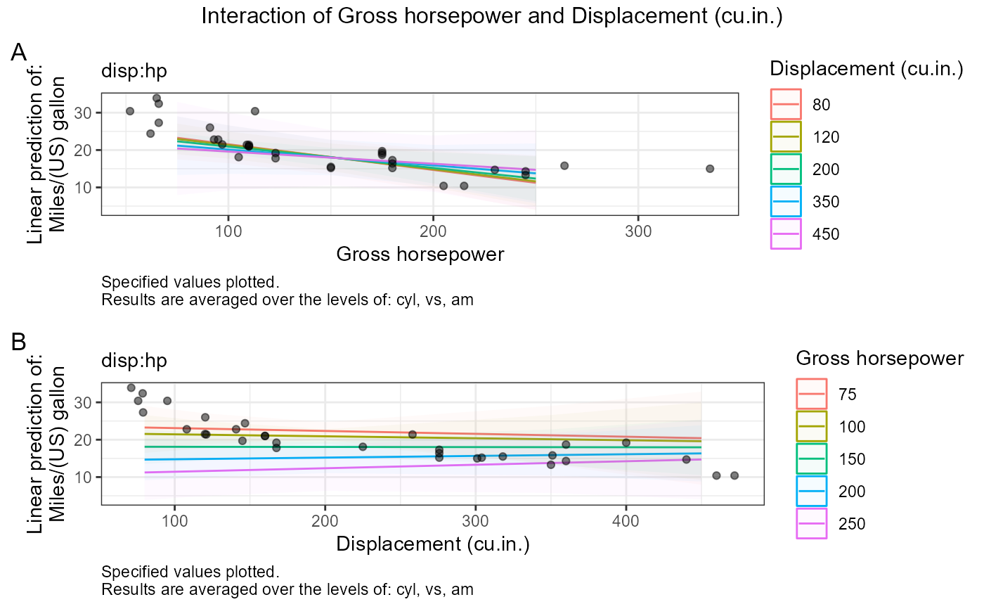
 # one specific numeric:numeric contrast with specified values
fit_contrasts <-
e_plot_model_contrasts(
fit = fit
, dat_cont = dat_cont
, choose_contrasts = "disp:hp"
, sw_table_in_plot = TRUE
, adjust_method = c("none", "tukey", "scheffe", "sidak", "bonferroni"
, "dunnettx", "mvt")[4] # see ?emmeans::summary.emmGrid
, CI_level = 0.95
, sw_glm_scale = c("link", "response")[1]
, sw_print = FALSE
, sw_marginal_even_if_interaction = TRUE
, sw_TWI_plots_keep = c("singles", "both", "all")[3]
, sw_TWI_both_orientation = c("tall", "wide")[1]
, sw_plot_quantiles_values = c("quantiles", "values")[2] # for numeric:numeric plots
, plot_quantiles = c(0.05, 0.25, 0.50, 0.75, 0.95) # for numeric:numeric plots
, sw_quantile_type = 1
, plot_values = list(hp = c(75, 100, 150, 200, 250)
, disp = c(80, 120, 200, 350, 450)) # for numeric:numeric plots
)
fit_contrasts$plots$`disp:hp`$both
# one specific numeric:numeric contrast with specified values
fit_contrasts <-
e_plot_model_contrasts(
fit = fit
, dat_cont = dat_cont
, choose_contrasts = "disp:hp"
, sw_table_in_plot = TRUE
, adjust_method = c("none", "tukey", "scheffe", "sidak", "bonferroni"
, "dunnettx", "mvt")[4] # see ?emmeans::summary.emmGrid
, CI_level = 0.95
, sw_glm_scale = c("link", "response")[1]
, sw_print = FALSE
, sw_marginal_even_if_interaction = TRUE
, sw_TWI_plots_keep = c("singles", "both", "all")[3]
, sw_TWI_both_orientation = c("tall", "wide")[1]
, sw_plot_quantiles_values = c("quantiles", "values")[2] # for numeric:numeric plots
, plot_quantiles = c(0.05, 0.25, 0.50, 0.75, 0.95) # for numeric:numeric plots
, sw_quantile_type = 1
, plot_values = list(hp = c(75, 100, 150, 200, 250)
, disp = c(80, 120, 200, 350, 450)) # for numeric:numeric plots
)
fit_contrasts$plots$`disp:hp`$both
 ## GLM on logit and probability scales
dat_cont <-
dat_cont %>%
dplyr::mutate(
am_01 =
dplyr::case_when(
am == "manual" ~ 0
, am == "automatic" ~ 1
)
)
labelled::var_label(dat_cont[["am_01"]]) <- labelled::var_label(dat_cont[["am"]])
# numeric:factor interaction
fit_glm <-
glm(
cbind(am_01, 1 - am_01) ~
vs + hp + vs:hp
, family = binomial
, data = dat_cont
)
car::Anova(fit_glm, type = 3)
#> Analysis of Deviance Table (Type III tests)
#>
#> Response: cbind(am_01, 1 - am_01)
#> LR Chisq Df Pr(>Chisq)
#> vs 1.78742 1 0.1812
#> hp 0.21115 1 0.6459
#> vs:hp 2.23005 1 0.1353
summary(fit_glm)
#>
#> Call:
#> glm(formula = cbind(am_01, 1 - am_01) ~ vs + hp + vs:hp, family = binomial,
#> data = dat_cont)
#>
#> Deviance Residuals:
#> Min 1Q Median 3Q Max
#> -1.7489 -1.2260 0.8176 0.9134 1.7682
#>
#> Coefficients:
#> Estimate Std. Error z value Pr(>|z|)
#> (Intercept) -0.058088 1.714742 -0.034 0.973
#> vsstraight -4.022917 3.155368 -1.275 0.202
#> hp 0.004009 0.008861 0.452 0.651
#> vsstraight:hp 0.040392 0.029123 1.387 0.165
#>
#> (Dispersion parameter for binomial family taken to be 1)
#>
#> Null deviance: 43.23 on 31 degrees of freedom
#> Residual deviance: 38.98 on 28 degrees of freedom
#> AIC: 46.98
#>
#> Number of Fisher Scoring iterations: 4
#>
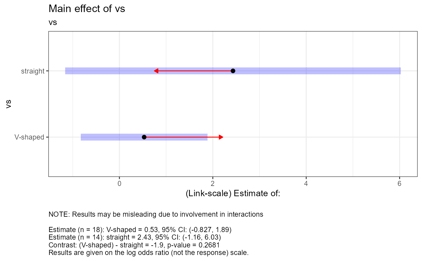
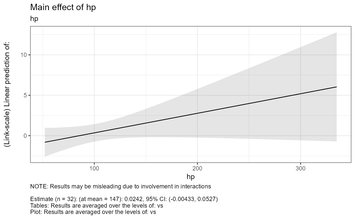
# all contrasts from model, logit scale
fit_contrasts <-
e_plot_model_contrasts(
fit = fit_glm
, dat_cont = dat_cont
, sw_glm_scale = c("link", "response")[1]
, sw_print = FALSE
, sw_marginal_even_if_interaction = TRUE
, sw_TWI_plots_keep = "both"
)
#> e_plot_model_contrasts: Continuing with "vs" even though involved in interactions.
#> NOTE: Results may be misleading due to involvement in interactions
#> e_plot_model_contrasts: Continuing with "hp" even though involved in interactions.
#> NOTE: Results may be misleading due to involvement in interactions
#> NOTE: Results may be misleading due to involvement in interactions
fit_contrasts
#> $tables
#> $tables$vs
#> $tables$vs$est
#> vs emmean SE df asymp.LCL asymp.UCL
#> V-shaped 0.53 0.607 Inf -0.827 1.89
#> straight 2.43 1.607 Inf -1.161 6.03
#>
#> Results are given on the logit (not the response) scale.
#> Confidence level used: 0.95
#> Conf-level adjustment: sidak method for 2 estimates
#>
#> $tables$vs$cont
#> contrast estimate SE df z.ratio p.value
#> (V-shaped) - straight -1.9 1.72 Inf -1.107 0.2681
#>
#> Results are given on the log odds ratio (not the response) scale.
#>
#>
#> $tables$hp
#> $tables$hp$est
#> hp hp.trend SE df asymp.LCL asymp.UCL
#> 147 0.0242 0.0146 Inf -0.00433 0.0527
#>
#> Results are averaged over the levels of: vs
#> Confidence level used: 0.95
#>
#>
#> $tables$`vs:hp`
#> $tables$`vs:hp`$est
#> vs hp.trend SE df asymp.LCL asymp.UCL
#> V-shaped 0.00401 0.00886 Inf -0.01336 0.0214
#> straight 0.04440 0.02774 Inf -0.00997 0.0988
#>
#> Confidence level used: 0.95
#>
#> $tables$`vs:hp`$cont
#> contrast estimate SE df z.ratio p.value
#> (V-shaped) - straight -0.0404 0.0291 Inf -1.387 0.1655
#>
#>
#>
#>
#> $plots
#> $plots$vs
## GLM on logit and probability scales
dat_cont <-
dat_cont %>%
dplyr::mutate(
am_01 =
dplyr::case_when(
am == "manual" ~ 0
, am == "automatic" ~ 1
)
)
labelled::var_label(dat_cont[["am_01"]]) <- labelled::var_label(dat_cont[["am"]])
# numeric:factor interaction
fit_glm <-
glm(
cbind(am_01, 1 - am_01) ~
vs + hp + vs:hp
, family = binomial
, data = dat_cont
)
car::Anova(fit_glm, type = 3)
#> Analysis of Deviance Table (Type III tests)
#>
#> Response: cbind(am_01, 1 - am_01)
#> LR Chisq Df Pr(>Chisq)
#> vs 1.78742 1 0.1812
#> hp 0.21115 1 0.6459
#> vs:hp 2.23005 1 0.1353
summary(fit_glm)
#>
#> Call:
#> glm(formula = cbind(am_01, 1 - am_01) ~ vs + hp + vs:hp, family = binomial,
#> data = dat_cont)
#>
#> Deviance Residuals:
#> Min 1Q Median 3Q Max
#> -1.7489 -1.2260 0.8176 0.9134 1.7682
#>
#> Coefficients:
#> Estimate Std. Error z value Pr(>|z|)
#> (Intercept) -0.058088 1.714742 -0.034 0.973
#> vsstraight -4.022917 3.155368 -1.275 0.202
#> hp 0.004009 0.008861 0.452 0.651
#> vsstraight:hp 0.040392 0.029123 1.387 0.165
#>
#> (Dispersion parameter for binomial family taken to be 1)
#>
#> Null deviance: 43.23 on 31 degrees of freedom
#> Residual deviance: 38.98 on 28 degrees of freedom
#> AIC: 46.98
#>
#> Number of Fisher Scoring iterations: 4
#>
# all contrasts from model, logit scale
fit_contrasts <-
e_plot_model_contrasts(
fit = fit_glm
, dat_cont = dat_cont
, sw_glm_scale = c("link", "response")[1]
, sw_print = FALSE
, sw_marginal_even_if_interaction = TRUE
, sw_TWI_plots_keep = "both"
)
#> e_plot_model_contrasts: Continuing with "vs" even though involved in interactions.
#> NOTE: Results may be misleading due to involvement in interactions
#> e_plot_model_contrasts: Continuing with "hp" even though involved in interactions.
#> NOTE: Results may be misleading due to involvement in interactions
#> NOTE: Results may be misleading due to involvement in interactions
fit_contrasts
#> $tables
#> $tables$vs
#> $tables$vs$est
#> vs emmean SE df asymp.LCL asymp.UCL
#> V-shaped 0.53 0.607 Inf -0.827 1.89
#> straight 2.43 1.607 Inf -1.161 6.03
#>
#> Results are given on the logit (not the response) scale.
#> Confidence level used: 0.95
#> Conf-level adjustment: sidak method for 2 estimates
#>
#> $tables$vs$cont
#> contrast estimate SE df z.ratio p.value
#> (V-shaped) - straight -1.9 1.72 Inf -1.107 0.2681
#>
#> Results are given on the log odds ratio (not the response) scale.
#>
#>
#> $tables$hp
#> $tables$hp$est
#> hp hp.trend SE df asymp.LCL asymp.UCL
#> 147 0.0242 0.0146 Inf -0.00433 0.0527
#>
#> Results are averaged over the levels of: vs
#> Confidence level used: 0.95
#>
#>
#> $tables$`vs:hp`
#> $tables$`vs:hp`$est
#> vs hp.trend SE df asymp.LCL asymp.UCL
#> V-shaped 0.00401 0.00886 Inf -0.01336 0.0214
#> straight 0.04440 0.02774 Inf -0.00997 0.0988
#>
#> Confidence level used: 0.95
#>
#> $tables$`vs:hp`$cont
#> contrast estimate SE df z.ratio p.value
#> (V-shaped) - straight -0.0404 0.0291 Inf -1.387 0.1655
#>
#>
#>
#>
#> $plots
#> $plots$vs
 #>
#> $plots$hp
#>
#> $plots$hp
 #>
#> $plots$`vs:hp`
#> $plots$`vs:hp`$both
#>
#> $plots$`vs:hp`
#> $plots$`vs:hp`$both
 #>
#>
#>
#> $text
#> $text$vs
#> $text$vs[[1]]
#> [1] "NOTE: Results may be misleading due to involvement in interactions"
#> [2] ""
#> [3] "Estimate (n = 18): V-shaped = 0.53, 95% CI: (-0.827, 1.89)"
#> [4] "Estimate (n = 14): straight = 2.43, 95% CI: (-1.16, 6.03)"
#> [5] "Contrast: (V-shaped) - straight = -1.9, p-value = 0.2681"
#> [6] "Results are given on the log odds ratio (not the response) scale."
#>
#>
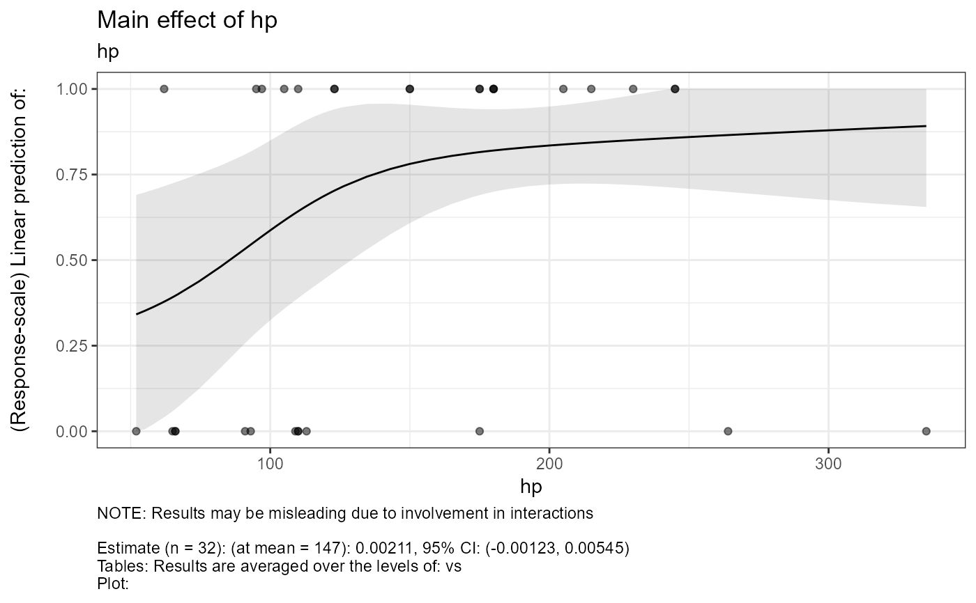
#> $text$hp
#> $text$hp[[1]]
#> [1] "NOTE: Results may be misleading due to involvement in interactions"
#> [2] ""
#> [3] "Estimate (n = 32): (at mean = 147): 0.0242, 95% CI: (-0.00433, 0.0527)"
#> [4] "Tables: Results are averaged over the levels of: vs"
#> [5] "Plot: Results are averaged over the levels of: vs"
#>
#> $text$hp[[2]]
#> [1] "NOTE: Results may be misleading due to involvement in interactions"
#> [2] ""
#> [3] "Estimate (n = 32): (at mean = 147): 0.0242, 95% CI: (-0.00433, 0.0527)"
#> [4] "Tables: Confidence level used: 0.95"
#> [5] "Plot: Results are given on the logit (not the response) scale."
#>
#> $text$hp[[3]]
#> [1] "NOTE: Results may be misleading due to involvement in interactions"
#> [2] ""
#> [3] "Estimate (n = 32): (at mean = 147): 0.0242, 95% CI: (-0.00433, 0.0527)"
#> [4] "Tables: Results are averaged over the levels of: vs"
#> [5] "Plot: Confidence level used: 0.95"
#>
#>
#> $text$`vs:hp`
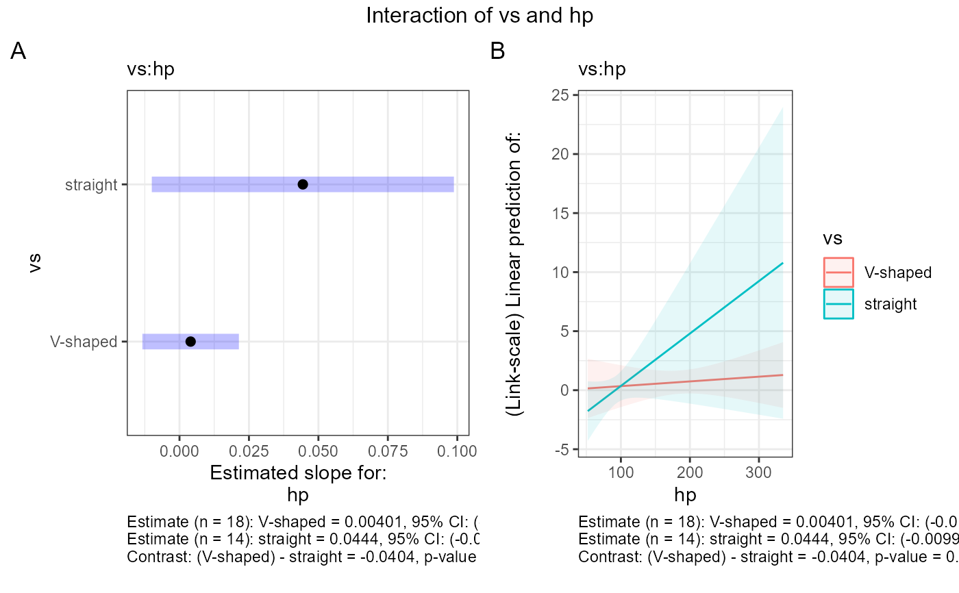
#> $text$`vs:hp`[[1]]
#> $text$`vs:hp`[[1]][[1]]
#> [1] "Estimate (n = 18): V-shaped = 0.00401, 95% CI: (-0.0134, 0.0214)"
#> [2] "Estimate (n = 14): straight = 0.0444, 95% CI: (-0.00997, 0.0988)"
#> [3] "Contrast: (V-shaped) - straight = -0.0404, p-value = 0.1655"
#> [4] ""
#>
#>
#> $text$`vs:hp`[[2]]
#> $text$`vs:hp`[[2]][[1]]
#> [1] "Estimate (n = 18): V-shaped = 0.00401, 95% CI: (-0.0134, 0.0214)"
#> [2] "Estimate (n = 14): straight = 0.0444, 95% CI: (-0.00997, 0.0988)"
#> [3] "Contrast: (V-shaped) - straight = -0.0404, p-value = 0.1655"
#> [4] ""
#>
#>
#>
#>
# all contrasts from model, probability scale
fit_contrasts <-
e_plot_model_contrasts(
fit = fit_glm
, dat_cont = dat_cont
, sw_glm_scale = c("link", "response")[2]
, sw_print = FALSE
, sw_marginal_even_if_interaction = TRUE
, sw_TWI_plots_keep = "both"
)
#> e_plot_model_contrasts: Continuing with "vs" even though involved in interactions.
#> NOTE: Results may be misleading due to involvement in interactions
#> e_plot_model_contrasts: Continuing with "hp" even though involved in interactions.
#> NOTE: Results may be misleading due to involvement in interactions
#> NOTE: Results may be misleading due to involvement in interactions
fit_contrasts
#> $tables
#> $tables$vs
#> $tables$vs$est
#> vs prob SE df asymp.LCL asymp.UCL
#> V-shaped 0.629 0.142 Inf 0.304 0.868
#> straight 0.919 0.119 Inf 0.238 0.998
#>
#> Confidence level used: 0.95
#> Conf-level adjustment: sidak method for 2 estimates
#> Intervals are back-transformed from the logit scale
#>
#> $tables$vs$cont
#> contrast odds.ratio SE df null z.ratio p.value
#> (V-shaped) / straight 0.149 0.256 Inf 1 -1.107 0.2681
#>
#> Tests are performed on the log odds ratio scale
#>
#>
#> $tables$hp
#> $tables$hp$est
#> hp hp.trend SE df asymp.LCL asymp.UCL
#> 147 0.00211 0.0017 Inf -0.00123 0.00545
#>
#> Results are averaged over the levels of: vs
#> Confidence level used: 0.95
#>
#>
#> $tables$`vs:hp`
#> $tables$`vs:hp`$est
#> vs hp.trend SE df asymp.LCL asymp.UCL
#> V-shaped 0.000935 0.00215 Inf -0.00328 0.00515
#> straight 0.003279 0.00265 Inf -0.00191 0.00846
#>
#> Confidence level used: 0.95
#>
#> $tables$`vs:hp`$cont
#> contrast estimate SE df z.ratio p.value
#> (V-shaped) - straight -0.00234 0.00341 Inf -0.687 0.4918
#>
#>
#>
#>
#> $plots
#> $plots$vs
#>
#>
#>
#> $text
#> $text$vs
#> $text$vs[[1]]
#> [1] "NOTE: Results may be misleading due to involvement in interactions"
#> [2] ""
#> [3] "Estimate (n = 18): V-shaped = 0.53, 95% CI: (-0.827, 1.89)"
#> [4] "Estimate (n = 14): straight = 2.43, 95% CI: (-1.16, 6.03)"
#> [5] "Contrast: (V-shaped) - straight = -1.9, p-value = 0.2681"
#> [6] "Results are given on the log odds ratio (not the response) scale."
#>
#>
#> $text$hp
#> $text$hp[[1]]
#> [1] "NOTE: Results may be misleading due to involvement in interactions"
#> [2] ""
#> [3] "Estimate (n = 32): (at mean = 147): 0.0242, 95% CI: (-0.00433, 0.0527)"
#> [4] "Tables: Results are averaged over the levels of: vs"
#> [5] "Plot: Results are averaged over the levels of: vs"
#>
#> $text$hp[[2]]
#> [1] "NOTE: Results may be misleading due to involvement in interactions"
#> [2] ""
#> [3] "Estimate (n = 32): (at mean = 147): 0.0242, 95% CI: (-0.00433, 0.0527)"
#> [4] "Tables: Confidence level used: 0.95"
#> [5] "Plot: Results are given on the logit (not the response) scale."
#>
#> $text$hp[[3]]
#> [1] "NOTE: Results may be misleading due to involvement in interactions"
#> [2] ""
#> [3] "Estimate (n = 32): (at mean = 147): 0.0242, 95% CI: (-0.00433, 0.0527)"
#> [4] "Tables: Results are averaged over the levels of: vs"
#> [5] "Plot: Confidence level used: 0.95"
#>
#>
#> $text$`vs:hp`
#> $text$`vs:hp`[[1]]
#> $text$`vs:hp`[[1]][[1]]
#> [1] "Estimate (n = 18): V-shaped = 0.00401, 95% CI: (-0.0134, 0.0214)"
#> [2] "Estimate (n = 14): straight = 0.0444, 95% CI: (-0.00997, 0.0988)"
#> [3] "Contrast: (V-shaped) - straight = -0.0404, p-value = 0.1655"
#> [4] ""
#>
#>
#> $text$`vs:hp`[[2]]
#> $text$`vs:hp`[[2]][[1]]
#> [1] "Estimate (n = 18): V-shaped = 0.00401, 95% CI: (-0.0134, 0.0214)"
#> [2] "Estimate (n = 14): straight = 0.0444, 95% CI: (-0.00997, 0.0988)"
#> [3] "Contrast: (V-shaped) - straight = -0.0404, p-value = 0.1655"
#> [4] ""
#>
#>
#>
#>
# all contrasts from model, probability scale
fit_contrasts <-
e_plot_model_contrasts(
fit = fit_glm
, dat_cont = dat_cont
, sw_glm_scale = c("link", "response")[2]
, sw_print = FALSE
, sw_marginal_even_if_interaction = TRUE
, sw_TWI_plots_keep = "both"
)
#> e_plot_model_contrasts: Continuing with "vs" even though involved in interactions.
#> NOTE: Results may be misleading due to involvement in interactions
#> e_plot_model_contrasts: Continuing with "hp" even though involved in interactions.
#> NOTE: Results may be misleading due to involvement in interactions
#> NOTE: Results may be misleading due to involvement in interactions
fit_contrasts
#> $tables
#> $tables$vs
#> $tables$vs$est
#> vs prob SE df asymp.LCL asymp.UCL
#> V-shaped 0.629 0.142 Inf 0.304 0.868
#> straight 0.919 0.119 Inf 0.238 0.998
#>
#> Confidence level used: 0.95
#> Conf-level adjustment: sidak method for 2 estimates
#> Intervals are back-transformed from the logit scale
#>
#> $tables$vs$cont
#> contrast odds.ratio SE df null z.ratio p.value
#> (V-shaped) / straight 0.149 0.256 Inf 1 -1.107 0.2681
#>
#> Tests are performed on the log odds ratio scale
#>
#>
#> $tables$hp
#> $tables$hp$est
#> hp hp.trend SE df asymp.LCL asymp.UCL
#> 147 0.00211 0.0017 Inf -0.00123 0.00545
#>
#> Results are averaged over the levels of: vs
#> Confidence level used: 0.95
#>
#>
#> $tables$`vs:hp`
#> $tables$`vs:hp`$est
#> vs hp.trend SE df asymp.LCL asymp.UCL
#> V-shaped 0.000935 0.00215 Inf -0.00328 0.00515
#> straight 0.003279 0.00265 Inf -0.00191 0.00846
#>
#> Confidence level used: 0.95
#>
#> $tables$`vs:hp`$cont
#> contrast estimate SE df z.ratio p.value
#> (V-shaped) - straight -0.00234 0.00341 Inf -0.687 0.4918
#>
#>
#>
#>
#> $plots
#> $plots$vs
 #>
#> $plots$hp
#>
#> $plots$hp
 #>
#> $plots$`vs:hp`
#> $plots$`vs:hp`$both
#>
#> $plots$`vs:hp`
#> $plots$`vs:hp`$both
 #>
#>
#>
#> $text
#> $text$vs
#> $text$vs[[1]]
#> [1] "NOTE: Results may be misleading due to involvement in interactions"
#> [2] ""
#> [3] "Estimate (n = 18): V-shaped = 0.629, 95% CI: (0.304, 0.868)"
#> [4] "Estimate (n = 14): straight = 0.919, 95% CI: (0.238, 0.998)"
#> [5] "Contrast: (V-shaped) / straight = 0.149, p-value = 0.2681"
#> [6] "Tests are performed on the log odds ratio scale"
#>
#>
#> $text$hp
#> $text$hp[[1]]
#> [1] "NOTE: Results may be misleading due to involvement in interactions"
#> [2] ""
#> [3] "Estimate (n = 32): (at mean = 147): 0.00211, 95% CI: (-0.00123, 0.00545)"
#> [4] "Tables: Results are averaged over the levels of: vs"
#> [5] "Plot: "
#>
#> $text$hp[[2]]
#> [1] "NOTE: Results may be misleading due to involvement in interactions"
#> [2] ""
#> [3] "Estimate (n = 32): (at mean = 147): 0.00211, 95% CI: (-0.00123, 0.00545)"
#> [4] "Tables: Confidence level used: 0.95"
#> [5] "Plot: "
#>
#>
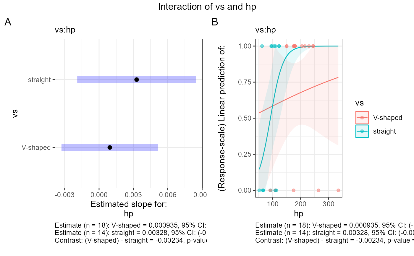
#> $text$`vs:hp`
#> $text$`vs:hp`[[1]]
#> $text$`vs:hp`[[1]][[1]]
#> [1] "Estimate (n = 18): V-shaped = 0.000935, 95% CI: (-0.00328, 0.00515)"
#> [2] "Estimate (n = 14): straight = 0.00328, 95% CI: (-0.00191, 0.00846)"
#> [3] "Contrast: (V-shaped) - straight = -0.00234, p-value = 0.4918"
#> [4] ""
#>
#>
#> $text$`vs:hp`[[2]]
#> $text$`vs:hp`[[2]][[1]]
#> [1] "Estimate (n = 18): V-shaped = 0.000935, 95% CI: (-0.00328, 0.00515)"
#> [2] "Estimate (n = 14): straight = 0.00328, 95% CI: (-0.00191, 0.00846)"
#> [3] "Contrast: (V-shaped) - straight = -0.00234, p-value = 0.4918"
#> [4] ""
#>
#>
#>
#>
# numeric:numeric interaction
fit_glm <-
glm(
cbind(am_01, 1 - am_01) ~
disp + hp + disp:hp
, family = binomial
, data = dat_cont
)
car::Anova(fit_glm, type = 3)
#> Analysis of Deviance Table (Type III tests)
#>
#> Response: cbind(am_01, 1 - am_01)
#> LR Chisq Df Pr(>Chisq)
#> disp 17.3730 1 3.072e-05 ***
#> hp 0.1824 1 0.6693
#> disp:hp 2.4178 1 0.1200
#> ---
#> Signif. codes: 0 '***' 0.001 '**' 0.01 '*' 0.05 '.' 0.1 ' ' 1
summary(fit_glm)
#>
#> Call:
#> glm(formula = cbind(am_01, 1 - am_01) ~ disp + hp + disp:hp,
#> family = binomial, data = dat_cont)
#>
#> Deviance Residuals:
#> Min 1Q Median 3Q Max
#> -1.64090 -0.21860 0.00604 0.18884 1.88968
#>
#> Coefficients:
#> Estimate Std. Error z value Pr(>|z|)
#> (Intercept) -9.3246479 6.8384757 -1.364 0.1727
#> disp 0.1138638 0.0482517 2.360 0.0183 *
#> hp -0.0312992 0.0794230 -0.394 0.6935
#> disp:hp -0.0002503 0.0001947 -1.285 0.1987
#> ---
#> Signif. codes: 0 '***' 0.001 '**' 0.01 '*' 0.05 '.' 0.1 ' ' 1
#>
#> (Dispersion parameter for binomial family taken to be 1)
#>
#> Null deviance: 43.230 on 31 degrees of freedom
#> Residual deviance: 14.295 on 28 degrees of freedom
#> AIC: 22.295
#>
#> Number of Fisher Scoring iterations: 8
#>
fit_contrasts <-
e_plot_model_contrasts(
fit = fit_glm
, dat_cont = dat_cont
, sw_glm_scale = c("link", "response")[2]
, sw_print = FALSE
, sw_TWI_plots_keep = "both"
)
#> e_plot_model_contrasts: Skipping "disp" since involved in interactions.
#> e_plot_model_contrasts: Skipping "hp" since involved in interactions.
fit_contrasts
#> $tables
#> list()
#>
#> $plots
#> $plots$`disp:hp`
#> $plots$`disp:hp`$both
#>
#>
#>
#> $text
#> $text$vs
#> $text$vs[[1]]
#> [1] "NOTE: Results may be misleading due to involvement in interactions"
#> [2] ""
#> [3] "Estimate (n = 18): V-shaped = 0.629, 95% CI: (0.304, 0.868)"
#> [4] "Estimate (n = 14): straight = 0.919, 95% CI: (0.238, 0.998)"
#> [5] "Contrast: (V-shaped) / straight = 0.149, p-value = 0.2681"
#> [6] "Tests are performed on the log odds ratio scale"
#>
#>
#> $text$hp
#> $text$hp[[1]]
#> [1] "NOTE: Results may be misleading due to involvement in interactions"
#> [2] ""
#> [3] "Estimate (n = 32): (at mean = 147): 0.00211, 95% CI: (-0.00123, 0.00545)"
#> [4] "Tables: Results are averaged over the levels of: vs"
#> [5] "Plot: "
#>
#> $text$hp[[2]]
#> [1] "NOTE: Results may be misleading due to involvement in interactions"
#> [2] ""
#> [3] "Estimate (n = 32): (at mean = 147): 0.00211, 95% CI: (-0.00123, 0.00545)"
#> [4] "Tables: Confidence level used: 0.95"
#> [5] "Plot: "
#>
#>
#> $text$`vs:hp`
#> $text$`vs:hp`[[1]]
#> $text$`vs:hp`[[1]][[1]]
#> [1] "Estimate (n = 18): V-shaped = 0.000935, 95% CI: (-0.00328, 0.00515)"
#> [2] "Estimate (n = 14): straight = 0.00328, 95% CI: (-0.00191, 0.00846)"
#> [3] "Contrast: (V-shaped) - straight = -0.00234, p-value = 0.4918"
#> [4] ""
#>
#>
#> $text$`vs:hp`[[2]]
#> $text$`vs:hp`[[2]][[1]]
#> [1] "Estimate (n = 18): V-shaped = 0.000935, 95% CI: (-0.00328, 0.00515)"
#> [2] "Estimate (n = 14): straight = 0.00328, 95% CI: (-0.00191, 0.00846)"
#> [3] "Contrast: (V-shaped) - straight = -0.00234, p-value = 0.4918"
#> [4] ""
#>
#>
#>
#>
# numeric:numeric interaction
fit_glm <-
glm(
cbind(am_01, 1 - am_01) ~
disp + hp + disp:hp
, family = binomial
, data = dat_cont
)
car::Anova(fit_glm, type = 3)
#> Analysis of Deviance Table (Type III tests)
#>
#> Response: cbind(am_01, 1 - am_01)
#> LR Chisq Df Pr(>Chisq)
#> disp 17.3730 1 3.072e-05 ***
#> hp 0.1824 1 0.6693
#> disp:hp 2.4178 1 0.1200
#> ---
#> Signif. codes: 0 '***' 0.001 '**' 0.01 '*' 0.05 '.' 0.1 ' ' 1
summary(fit_glm)
#>
#> Call:
#> glm(formula = cbind(am_01, 1 - am_01) ~ disp + hp + disp:hp,
#> family = binomial, data = dat_cont)
#>
#> Deviance Residuals:
#> Min 1Q Median 3Q Max
#> -1.64090 -0.21860 0.00604 0.18884 1.88968
#>
#> Coefficients:
#> Estimate Std. Error z value Pr(>|z|)
#> (Intercept) -9.3246479 6.8384757 -1.364 0.1727
#> disp 0.1138638 0.0482517 2.360 0.0183 *
#> hp -0.0312992 0.0794230 -0.394 0.6935
#> disp:hp -0.0002503 0.0001947 -1.285 0.1987
#> ---
#> Signif. codes: 0 '***' 0.001 '**' 0.01 '*' 0.05 '.' 0.1 ' ' 1
#>
#> (Dispersion parameter for binomial family taken to be 1)
#>
#> Null deviance: 43.230 on 31 degrees of freedom
#> Residual deviance: 14.295 on 28 degrees of freedom
#> AIC: 22.295
#>
#> Number of Fisher Scoring iterations: 8
#>
fit_contrasts <-
e_plot_model_contrasts(
fit = fit_glm
, dat_cont = dat_cont
, sw_glm_scale = c("link", "response")[2]
, sw_print = FALSE
, sw_TWI_plots_keep = "both"
)
#> e_plot_model_contrasts: Skipping "disp" since involved in interactions.
#> e_plot_model_contrasts: Skipping "hp" since involved in interactions.
fit_contrasts
#> $tables
#> list()
#>
#> $plots
#> $plots$`disp:hp`
#> $plots$`disp:hp`$both
 #>
#>
#>
#> $text
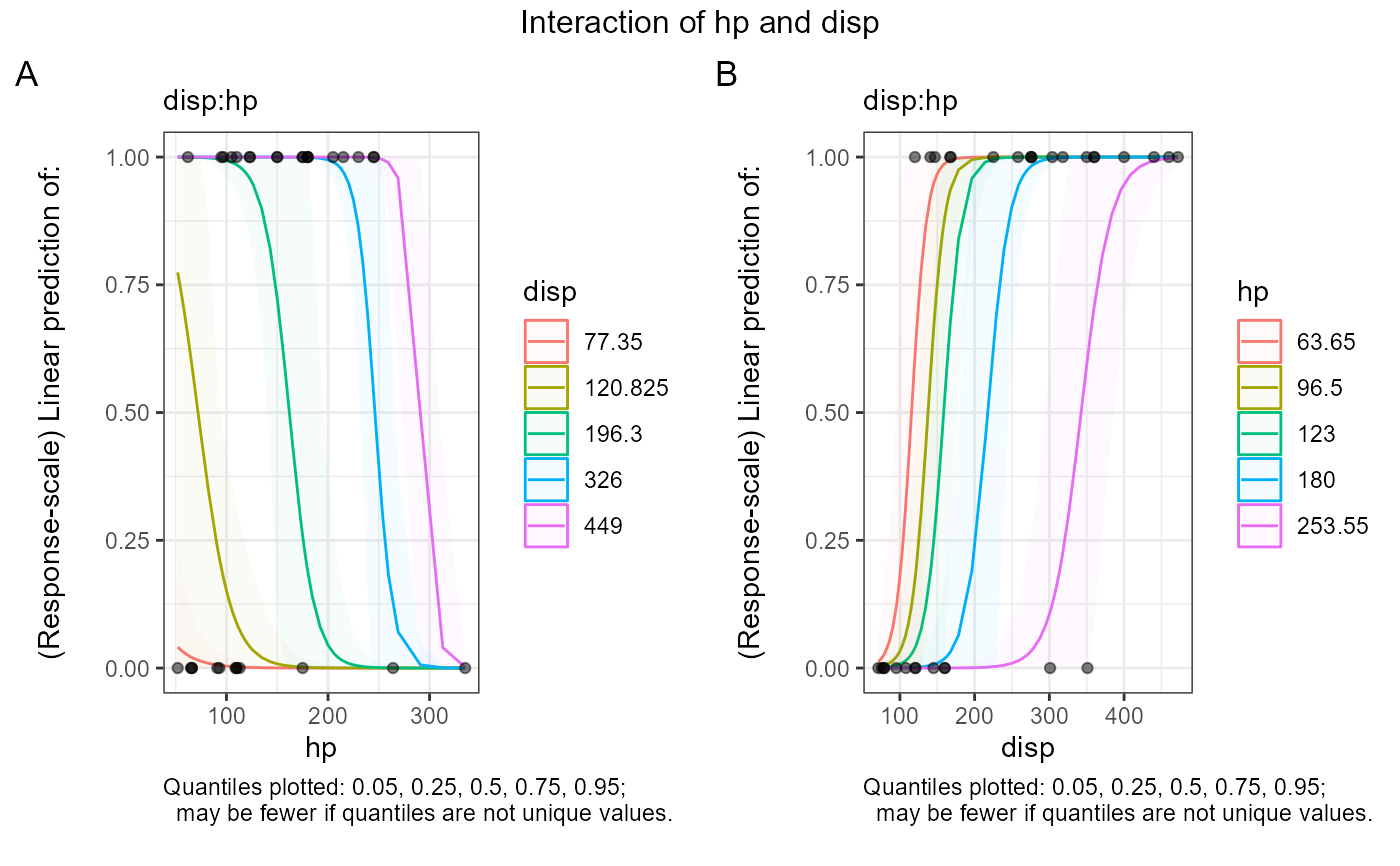
#> $text$`disp:hp`
#> $text$`disp:hp`[[1]]
#> $text$`disp:hp`[[1]][[1]]
#> [1] "Quantiles plotted: 0.05, 0.25, 0.5, 0.75, 0.95;"
#> [2] " may be fewer if quantiles are not unique values."
#> [3] ""
#>
#>
#> $text$`disp:hp`[[2]]
#> $text$`disp:hp`[[2]][[1]]
#> [1] "Quantiles plotted: 0.05, 0.25, 0.5, 0.75, 0.95;"
#> [2] " may be fewer if quantiles are not unique values."
#> [3] ""
#>
#>
#>
#>
# factor:factor interaction
fit_glm <-
glm(
cbind(am_01, 1 - am_01) ~
vs + cyl + vs:cyl
, family = binomial
, data = dat_cont
)
car::Anova(fit_glm) #, type = 3)
#> Warning: glm.fit: fitted probabilities numerically 0 or 1 occurred
#> Warning: glm.fit: fitted probabilities numerically 0 or 1 occurred
#> Warning: glm.fit: fitted probabilities numerically 0 or 1 occurred
#> Analysis of Deviance Table (Type II tests)
#>
#> Response: cbind(am_01, 1 - am_01)
#> LR Chisq Df Pr(>Chisq)
#> vs 10.234 1 0.001378 **
#> cyl 18.622 2 9.042e-05 ***
#> vs:cyl 0.000 1 1.000000
#> ---
#> Signif. codes: 0 '***' 0.001 '**' 0.01 '*' 0.05 '.' 0.1 ' ' 1
summary(fit_glm)
#>
#> Call:
#> glm(formula = cbind(am_01, 1 - am_01) ~ vs + cyl + vs:cyl, family = binomial,
#> data = dat_cont)
#>
#> Deviance Residuals:
#> Min 1Q Median 3Q Max
#> -1.97277 -0.84460 0.00013 0.55525 1.55176
#>
#> Coefficients: (1 not defined because of singularities)
#> Estimate Std. Error z value Pr(>|z|)
#> (Intercept) -1.857e+01 6.523e+03 -0.003 0.998
#> vsstraight 1.772e+01 6.523e+03 0.003 0.998
#> cylsix 1.191e-11 7.532e+03 0.000 1.000
#> cyleight 2.036e+01 6.523e+03 0.003 0.998
#> vsstraight:cylsix 1.941e+01 8.207e+03 0.002 0.998
#> vsstraight:cyleight NA NA NA NA
#>
#> (Dispersion parameter for binomial family taken to be 1)
#>
#> Null deviance: 43.230 on 31 degrees of freedom
#> Residual deviance: 23.701 on 27 degrees of freedom
#> AIC: 33.701
#>
#> Number of Fisher Scoring iterations: 17
#>
fit_contrasts <-
e_plot_model_contrasts(
fit = fit_glm
, dat_cont = dat_cont
, sw_glm_scale = c("link", "response")[2]
, sw_print = FALSE
, sw_TWI_plots_keep = "both"
)
#> e_plot_model_contrasts: Skipping "vs" since involved in interactions.
#> e_plot_model_contrasts: Skipping "cyl" since involved in interactions.
#> Warning: Comparison discrepancy in group "straight", four - six:
#> Target overlap = 0.9975, overlap on graph = -20.8762
#> Warning: Comparison discrepancy in group "straight", four - six:
#> Target overlap = 0.9975, overlap on graph = -21.2872
#> Warning: Removed 1 rows containing missing values (`geom_point()`).
#> Warning: Removed 1 rows containing missing values (`geom_segment()`).
#> Warning: Removed 1 rows containing missing values (`geom_point()`).
#> Warning: Removed 1 rows containing missing values (`geom_point()`).
#> Warning: Removed 1 rows containing missing values (`geom_segment()`).
#> Warning: Removed 1 rows containing missing values (`geom_point()`).
fit_contrasts
#> $tables
#> $tables$`vs:cyl`
#> $tables$`vs:cyl`$est
#> vs = V-shaped:
#> cyl prob SE df asymp.LCL asymp.UCL
#> four 0.00000 0.00005640 Inf 0.00000 1.00000
#> six 0.00000 0.00003256 Inf 0.00000 1.00000
#> eight 0.85714 0.09352195 Inf 0.49202 0.97380
#>
#> vs = straight:
#> cyl prob SE df asymp.LCL asymp.UCL
#> four 0.30000 0.14491377 Inf 0.07621 0.69006
#> six 1.00000 0.00002820 Inf 0.00000 1.00000
#> eight nonEst NA NA NA NA
#>
#> Confidence level used: 0.95
#> Conf-level adjustment: sidak method for 3 estimates
#> Intervals are back-transformed from the logit scale
#>
#> $tables$`vs:cyl`$cont
#> vs = V-shaped:
#> contrast odds.ratio SE df null z.ratio p.value
#> four / six 1 7532 Inf 1 0.000 1.0000
#> four / eight 0 0 Inf 1 -0.003 1.0000
#> six / eight 0 0 Inf 1 -0.005 1.0000
#>
#> vs = straight:
#> contrast odds.ratio SE df null z.ratio p.value
#> four / six 0 0 Inf 1 -0.006 1.0000
#> four / eight nonEst NA NA 1 NA NA
#> six / eight nonEst NA NA 1 NA NA
#>
#> P value adjustment: sidak method for 3 tests
#> Tests are performed on the log odds ratio scale
#>
#>
#>
#> $plots
#> $plots$`vs:cyl`
#> $plots$`vs:cyl`$both
#>
#>
#>
#> $text
#> $text$`disp:hp`
#> $text$`disp:hp`[[1]]
#> $text$`disp:hp`[[1]][[1]]
#> [1] "Quantiles plotted: 0.05, 0.25, 0.5, 0.75, 0.95;"
#> [2] " may be fewer if quantiles are not unique values."
#> [3] ""
#>
#>
#> $text$`disp:hp`[[2]]
#> $text$`disp:hp`[[2]][[1]]
#> [1] "Quantiles plotted: 0.05, 0.25, 0.5, 0.75, 0.95;"
#> [2] " may be fewer if quantiles are not unique values."
#> [3] ""
#>
#>
#>
#>
# factor:factor interaction
fit_glm <-
glm(
cbind(am_01, 1 - am_01) ~
vs + cyl + vs:cyl
, family = binomial
, data = dat_cont
)
car::Anova(fit_glm) #, type = 3)
#> Warning: glm.fit: fitted probabilities numerically 0 or 1 occurred
#> Warning: glm.fit: fitted probabilities numerically 0 or 1 occurred
#> Warning: glm.fit: fitted probabilities numerically 0 or 1 occurred
#> Analysis of Deviance Table (Type II tests)
#>
#> Response: cbind(am_01, 1 - am_01)
#> LR Chisq Df Pr(>Chisq)
#> vs 10.234 1 0.001378 **
#> cyl 18.622 2 9.042e-05 ***
#> vs:cyl 0.000 1 1.000000
#> ---
#> Signif. codes: 0 '***' 0.001 '**' 0.01 '*' 0.05 '.' 0.1 ' ' 1
summary(fit_glm)
#>
#> Call:
#> glm(formula = cbind(am_01, 1 - am_01) ~ vs + cyl + vs:cyl, family = binomial,
#> data = dat_cont)
#>
#> Deviance Residuals:
#> Min 1Q Median 3Q Max
#> -1.97277 -0.84460 0.00013 0.55525 1.55176
#>
#> Coefficients: (1 not defined because of singularities)
#> Estimate Std. Error z value Pr(>|z|)
#> (Intercept) -1.857e+01 6.523e+03 -0.003 0.998
#> vsstraight 1.772e+01 6.523e+03 0.003 0.998
#> cylsix 1.191e-11 7.532e+03 0.000 1.000
#> cyleight 2.036e+01 6.523e+03 0.003 0.998
#> vsstraight:cylsix 1.941e+01 8.207e+03 0.002 0.998
#> vsstraight:cyleight NA NA NA NA
#>
#> (Dispersion parameter for binomial family taken to be 1)
#>
#> Null deviance: 43.230 on 31 degrees of freedom
#> Residual deviance: 23.701 on 27 degrees of freedom
#> AIC: 33.701
#>
#> Number of Fisher Scoring iterations: 17
#>
fit_contrasts <-
e_plot_model_contrasts(
fit = fit_glm
, dat_cont = dat_cont
, sw_glm_scale = c("link", "response")[2]
, sw_print = FALSE
, sw_TWI_plots_keep = "both"
)
#> e_plot_model_contrasts: Skipping "vs" since involved in interactions.
#> e_plot_model_contrasts: Skipping "cyl" since involved in interactions.
#> Warning: Comparison discrepancy in group "straight", four - six:
#> Target overlap = 0.9975, overlap on graph = -20.8762
#> Warning: Comparison discrepancy in group "straight", four - six:
#> Target overlap = 0.9975, overlap on graph = -21.2872
#> Warning: Removed 1 rows containing missing values (`geom_point()`).
#> Warning: Removed 1 rows containing missing values (`geom_segment()`).
#> Warning: Removed 1 rows containing missing values (`geom_point()`).
#> Warning: Removed 1 rows containing missing values (`geom_point()`).
#> Warning: Removed 1 rows containing missing values (`geom_segment()`).
#> Warning: Removed 1 rows containing missing values (`geom_point()`).
fit_contrasts
#> $tables
#> $tables$`vs:cyl`
#> $tables$`vs:cyl`$est
#> vs = V-shaped:
#> cyl prob SE df asymp.LCL asymp.UCL
#> four 0.00000 0.00005640 Inf 0.00000 1.00000
#> six 0.00000 0.00003256 Inf 0.00000 1.00000
#> eight 0.85714 0.09352195 Inf 0.49202 0.97380
#>
#> vs = straight:
#> cyl prob SE df asymp.LCL asymp.UCL
#> four 0.30000 0.14491377 Inf 0.07621 0.69006
#> six 1.00000 0.00002820 Inf 0.00000 1.00000
#> eight nonEst NA NA NA NA
#>
#> Confidence level used: 0.95
#> Conf-level adjustment: sidak method for 3 estimates
#> Intervals are back-transformed from the logit scale
#>
#> $tables$`vs:cyl`$cont
#> vs = V-shaped:
#> contrast odds.ratio SE df null z.ratio p.value
#> four / six 1 7532 Inf 1 0.000 1.0000
#> four / eight 0 0 Inf 1 -0.003 1.0000
#> six / eight 0 0 Inf 1 -0.005 1.0000
#>
#> vs = straight:
#> contrast odds.ratio SE df null z.ratio p.value
#> four / six 0 0 Inf 1 -0.006 1.0000
#> four / eight nonEst NA NA 1 NA NA
#> six / eight nonEst NA NA 1 NA NA
#>
#> P value adjustment: sidak method for 3 tests
#> Tests are performed on the log odds ratio scale
#>
#>
#>
#> $plots
#> $plots$`vs:cyl`
#> $plots$`vs:cyl`$both
 #>
#>
#>
#> $text
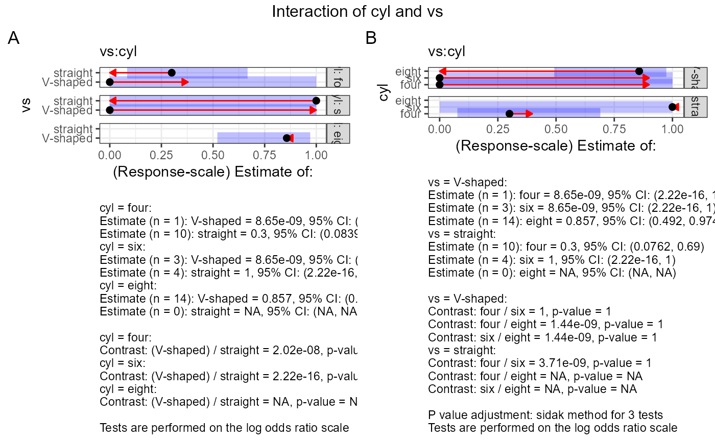
#> $text$`vs:cyl`
#> $text$`vs:cyl`[[1]]
#> $text$`vs:cyl`[[1]][[1]]
#> [1] "cyl = four:"
#> [2] "Estimate (n = 1): V-shaped = 8.65e-09, 95% CI: (2.22e-16, 1)"
#> [3] "Estimate (n = 10): straight = 0.3, 95% CI: (0.0839, 0.667)"
#> [4] "cyl = six:"
#> [5] "Estimate (n = 3): V-shaped = 8.65e-09, 95% CI: (2.22e-16, 1)"
#> [6] "Estimate (n = 4): straight = 1, 95% CI: (2.22e-16, 1)"
#> [7] "cyl = eight:"
#> [8] "Estimate (n = 14): V-shaped = 0.857, 95% CI: (0.521, 0.971)"
#> [9] "Estimate (n = 0): straight = NA, 95% CI: (NA, NA)"
#> [10] ""
#> [11] "cyl = four:"
#> [12] "Contrast: (V-shaped) / straight = 2.02e-08, p-value = 0.9978"
#> [13] "cyl = six:"
#> [14] "Contrast: (V-shaped) / straight = 2.22e-16, p-value = 0.9941"
#> [15] "cyl = eight:"
#> [16] "Contrast: (V-shaped) / straight = NA, p-value = NA"
#> [17] ""
#> [18] "Tests are performed on the log odds ratio scale"
#>
#>
#> $text$`vs:cyl`[[2]]
#> $text$`vs:cyl`[[2]][[1]]
#> [1] "vs = V-shaped:"
#> [2] "Estimate (n = 1): four = 8.65e-09, 95% CI: (2.22e-16, 1)"
#> [3] "Estimate (n = 3): six = 8.65e-09, 95% CI: (2.22e-16, 1)"
#> [4] "Estimate (n = 14): eight = 0.857, 95% CI: (0.492, 0.974)"
#> [5] "vs = straight:"
#> [6] "Estimate (n = 10): four = 0.3, 95% CI: (0.0762, 0.69)"
#> [7] "Estimate (n = 4): six = 1, 95% CI: (2.22e-16, 1)"
#> [8] "Estimate (n = 0): eight = NA, 95% CI: (NA, NA)"
#> [9] ""
#> [10] "vs = V-shaped:"
#> [11] "Contrast: four / six = 1, p-value = 1"
#> [12] "Contrast: four / eight = 1.44e-09, p-value = 1"
#> [13] "Contrast: six / eight = 1.44e-09, p-value = 1"
#> [14] "vs = straight:"
#> [15] "Contrast: four / six = 3.71e-09, p-value = 1"
#> [16] "Contrast: four / eight = NA, p-value = NA"
#> [17] "Contrast: six / eight = NA, p-value = NA"
#> [18] ""
#> [19] "P value adjustment: sidak method for 3 tests"
#> [20] "Tests are performed on the log odds ratio scale"
#>
#>
#>
#>
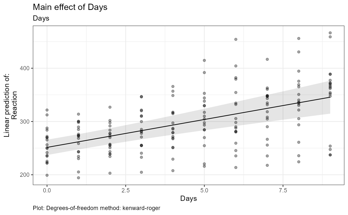
## lme4::lmer mixed-effects model
fit_lmer <-
lme4::lmer(
formula = Reaction ~ Days + (Days | Subject)
, data = lme4::sleepstudy
)
fit_lmer_contrasts <-
e_plot_model_contrasts(
fit = fit_lmer
, dat_cont = lme4::sleepstudy
, sw_print = FALSE
, sw_table_in_plot = FALSE
)
fit_lmer_contrasts
#> $tables
#> $tables$Days
#> $tables$Days$est
#> Days Days.trend SE df lower.CL upper.CL
#> 4.5 10.5 1.55 17 7.21 13.7
#>
#> Degrees-of-freedom method: kenward-roger
#> Confidence level used: 0.95
#>
#>
#>
#> $plots
#> $plots$Days
#>
#>
#>
#> $text
#> $text$`vs:cyl`
#> $text$`vs:cyl`[[1]]
#> $text$`vs:cyl`[[1]][[1]]
#> [1] "cyl = four:"
#> [2] "Estimate (n = 1): V-shaped = 8.65e-09, 95% CI: (2.22e-16, 1)"
#> [3] "Estimate (n = 10): straight = 0.3, 95% CI: (0.0839, 0.667)"
#> [4] "cyl = six:"
#> [5] "Estimate (n = 3): V-shaped = 8.65e-09, 95% CI: (2.22e-16, 1)"
#> [6] "Estimate (n = 4): straight = 1, 95% CI: (2.22e-16, 1)"
#> [7] "cyl = eight:"
#> [8] "Estimate (n = 14): V-shaped = 0.857, 95% CI: (0.521, 0.971)"
#> [9] "Estimate (n = 0): straight = NA, 95% CI: (NA, NA)"
#> [10] ""
#> [11] "cyl = four:"
#> [12] "Contrast: (V-shaped) / straight = 2.02e-08, p-value = 0.9978"
#> [13] "cyl = six:"
#> [14] "Contrast: (V-shaped) / straight = 2.22e-16, p-value = 0.9941"
#> [15] "cyl = eight:"
#> [16] "Contrast: (V-shaped) / straight = NA, p-value = NA"
#> [17] ""
#> [18] "Tests are performed on the log odds ratio scale"
#>
#>
#> $text$`vs:cyl`[[2]]
#> $text$`vs:cyl`[[2]][[1]]
#> [1] "vs = V-shaped:"
#> [2] "Estimate (n = 1): four = 8.65e-09, 95% CI: (2.22e-16, 1)"
#> [3] "Estimate (n = 3): six = 8.65e-09, 95% CI: (2.22e-16, 1)"
#> [4] "Estimate (n = 14): eight = 0.857, 95% CI: (0.492, 0.974)"
#> [5] "vs = straight:"
#> [6] "Estimate (n = 10): four = 0.3, 95% CI: (0.0762, 0.69)"
#> [7] "Estimate (n = 4): six = 1, 95% CI: (2.22e-16, 1)"
#> [8] "Estimate (n = 0): eight = NA, 95% CI: (NA, NA)"
#> [9] ""
#> [10] "vs = V-shaped:"
#> [11] "Contrast: four / six = 1, p-value = 1"
#> [12] "Contrast: four / eight = 1.44e-09, p-value = 1"
#> [13] "Contrast: six / eight = 1.44e-09, p-value = 1"
#> [14] "vs = straight:"
#> [15] "Contrast: four / six = 3.71e-09, p-value = 1"
#> [16] "Contrast: four / eight = NA, p-value = NA"
#> [17] "Contrast: six / eight = NA, p-value = NA"
#> [18] ""
#> [19] "P value adjustment: sidak method for 3 tests"
#> [20] "Tests are performed on the log odds ratio scale"
#>
#>
#>
#>
## lme4::lmer mixed-effects model
fit_lmer <-
lme4::lmer(
formula = Reaction ~ Days + (Days | Subject)
, data = lme4::sleepstudy
)
fit_lmer_contrasts <-
e_plot_model_contrasts(
fit = fit_lmer
, dat_cont = lme4::sleepstudy
, sw_print = FALSE
, sw_table_in_plot = FALSE
)
fit_lmer_contrasts
#> $tables
#> $tables$Days
#> $tables$Days$est
#> Days Days.trend SE df lower.CL upper.CL
#> 4.5 10.5 1.55 17 7.21 13.7
#>
#> Degrees-of-freedom method: kenward-roger
#> Confidence level used: 0.95
#>
#>
#>
#> $plots
#> $plots$Days
 #>
#>
#> $text
#> $text$Days
#> $text$Days[[1]]
#> [1] "Estimate (n = 180): (at mean = 4.5): 10.5, 95% CI: (7.21, 13.7)"
#> [2] "Tables: Degrees-of-freedom method: kenward-roger"
#> [3] "Plot: Degrees-of-freedom method: kenward-roger"
#>
#> $text$Days[[2]]
#> [1] "Estimate (n = 180): (at mean = 4.5): 10.5, 95% CI: (7.21, 13.7)"
#> [2] "Tables: Confidence level used: 0.95"
#> [3] "Plot: Confidence level used: 0.95"
#>
#>
#>
## lmerTest::as_lmerModLmerTest mixed-effects model
fit_lmer <-
lmerTest::as_lmerModLmerTest(fit_lmer)
fit_lmer_contrasts <-
e_plot_model_contrasts(
fit = fit_lmer
, dat_cont = lme4::sleepstudy
, sw_print = FALSE
, sw_table_in_plot = FALSE
)
fit_lmer_contrasts
#> $tables
#> $tables$Days
#> $tables$Days$est
#> Days Days.trend SE df lower.CL upper.CL
#> 4.5 10.5 1.55 17 7.21 13.7
#>
#> Degrees-of-freedom method: kenward-roger
#> Confidence level used: 0.95
#>
#>
#>
#> $plots
#> $plots$Days
#>
#>
#> $text
#> $text$Days
#> $text$Days[[1]]
#> [1] "Estimate (n = 180): (at mean = 4.5): 10.5, 95% CI: (7.21, 13.7)"
#> [2] "Tables: Degrees-of-freedom method: kenward-roger"
#> [3] "Plot: Degrees-of-freedom method: kenward-roger"
#>
#> $text$Days[[2]]
#> [1] "Estimate (n = 180): (at mean = 4.5): 10.5, 95% CI: (7.21, 13.7)"
#> [2] "Tables: Confidence level used: 0.95"
#> [3] "Plot: Confidence level used: 0.95"
#>
#>
#>
## lmerTest::as_lmerModLmerTest mixed-effects model
fit_lmer <-
lmerTest::as_lmerModLmerTest(fit_lmer)
fit_lmer_contrasts <-
e_plot_model_contrasts(
fit = fit_lmer
, dat_cont = lme4::sleepstudy
, sw_print = FALSE
, sw_table_in_plot = FALSE
)
fit_lmer_contrasts
#> $tables
#> $tables$Days
#> $tables$Days$est
#> Days Days.trend SE df lower.CL upper.CL
#> 4.5 10.5 1.55 17 7.21 13.7
#>
#> Degrees-of-freedom method: kenward-roger
#> Confidence level used: 0.95
#>
#>
#>
#> $plots
#> $plots$Days
 #>
#>
#> $text
#> $text$Days
#> $text$Days[[1]]
#> [1] "Estimate (n = 180): (at mean = 4.5): 10.5, 95% CI: (7.21, 13.7)"
#> [2] "Tables: Degrees-of-freedom method: kenward-roger"
#> [3] "Plot: Degrees-of-freedom method: kenward-roger"
#>
#> $text$Days[[2]]
#> [1] "Estimate (n = 180): (at mean = 4.5): 10.5, 95% CI: (7.21, 13.7)"
#> [2] "Tables: Confidence level used: 0.95"
#> [3] "Plot: Confidence level used: 0.95"
#>
#>
#>
#>
#>
#> $text
#> $text$Days
#> $text$Days[[1]]
#> [1] "Estimate (n = 180): (at mean = 4.5): 10.5, 95% CI: (7.21, 13.7)"
#> [2] "Tables: Degrees-of-freedom method: kenward-roger"
#> [3] "Plot: Degrees-of-freedom method: kenward-roger"
#>
#> $text$Days[[2]]
#> [1] "Estimate (n = 180): (at mean = 4.5): 10.5, 95% CI: (7.21, 13.7)"
#> [2] "Tables: Confidence level used: 0.95"
#> [3] "Plot: Confidence level used: 0.95"
#>
#>
#>