Plotting residual diagnostics for an lm() object.

e_plot_lm_diagnostics(
  fit = NULL,
  rc_mfrow = c(1, 3),
  which_plot = c(4, 6, 1),
  n_outliers = 3,
  sw_qqplot = TRUE,
  sw_boxcox = TRUE,
  sw_constant_var = TRUE,
  sw_collinearity = TRUE,
  sw_order_of_data = TRUE,
  sw_addedvar = TRUE,
  sw_plot_set = c(NA, "simple", "simpleAV", "all")[1]
)

Arguments

fit: linear model object returned by lm()
rc_mfrow: number of rows and columns for the graphic plot, default is c(1, 3); use "NA" for a single plot with 3 columns
which_plot: default plot numbers for lm()
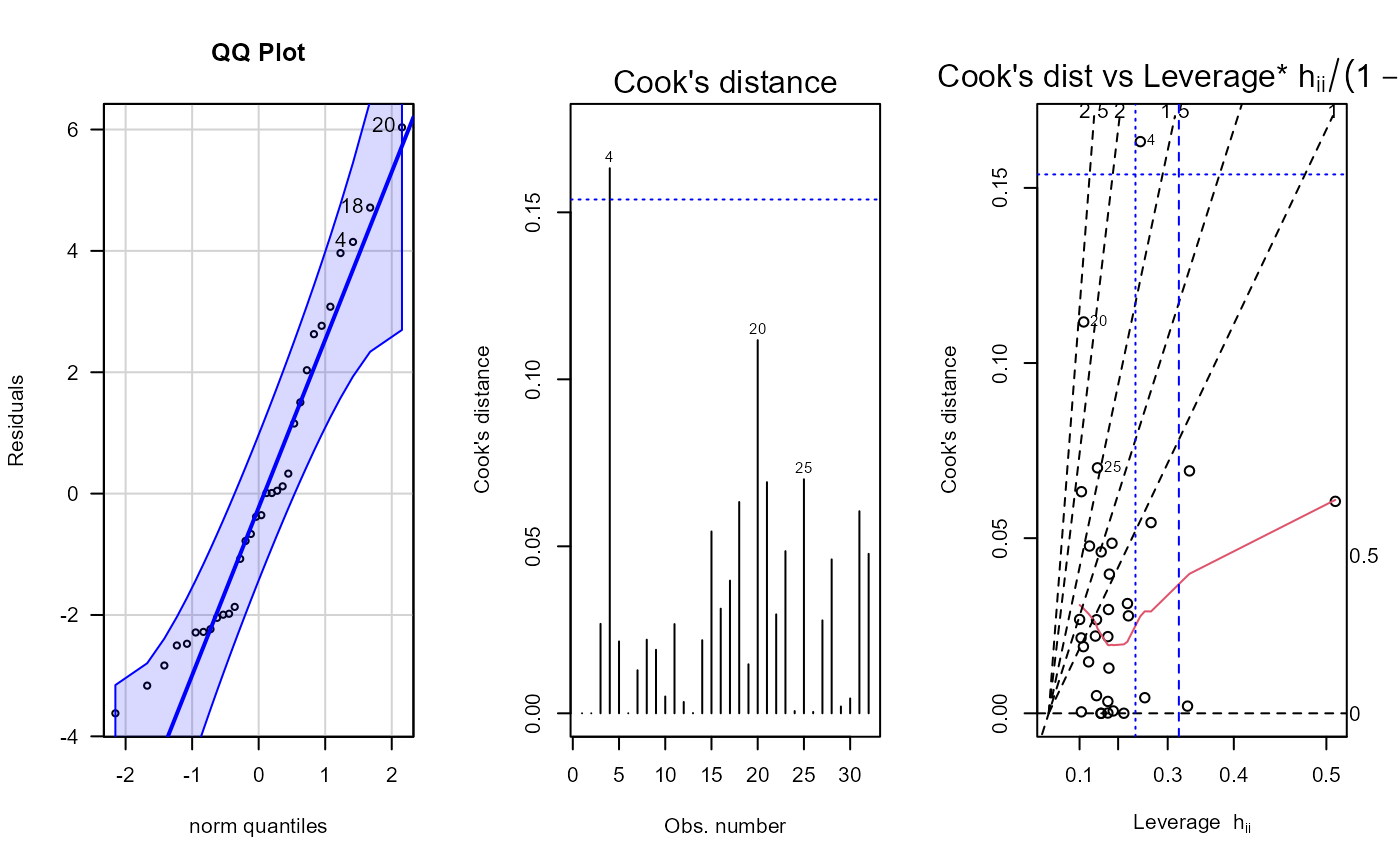
n_outliers: number to identify in plots from lm() and qqPlot()
sw_qqplot: T/F for whether to show the QQ-plot
sw_boxcox: T/F for whether to show Box-Cox transformation
sw_constant_var: T/F for whether to assess constant variance
sw_collinearity: T/F for whether to assess multicollinearity between predictor variables
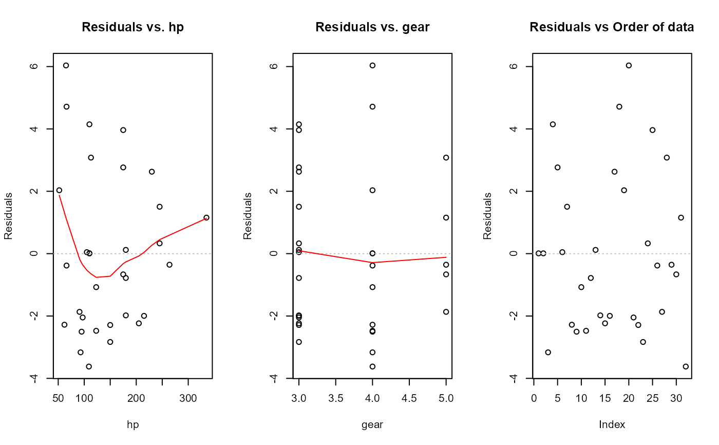
sw_order_of_data: T/F for whether to show residuals by order of data
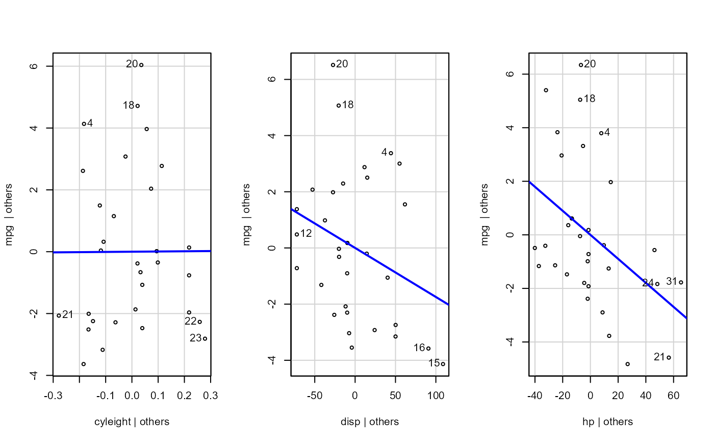
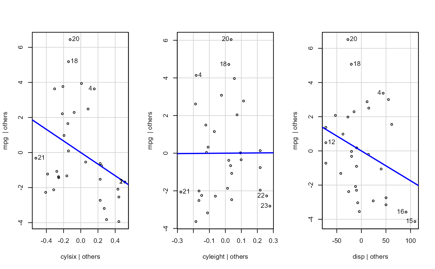
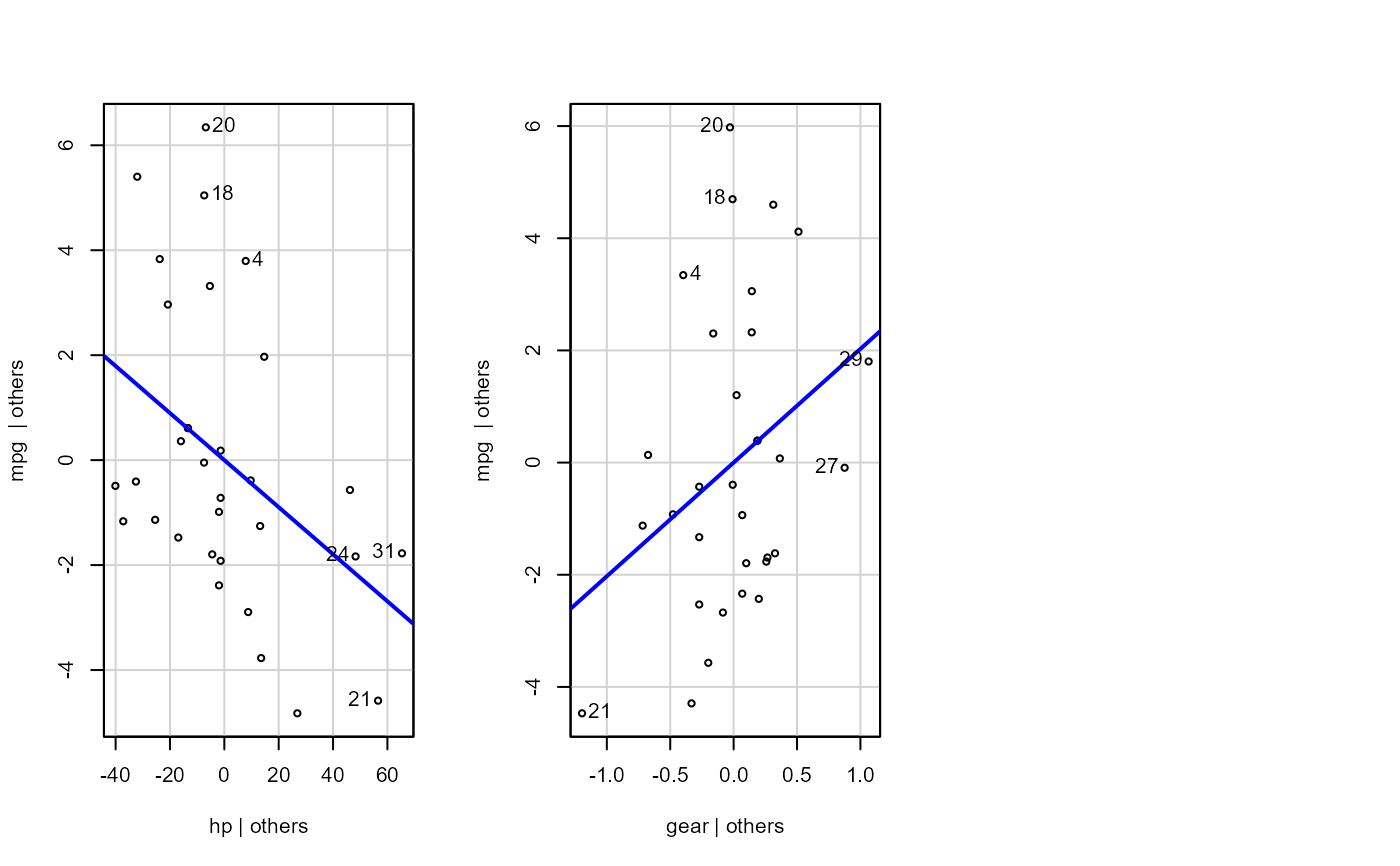
sw_addedvar: T/F for whether to show added-variables plot
sw_plot_set: NULL to accept other plot options, or "simple" to exclude boxcox, constant var, collinearity, order of data, and added-variable plots. "simpleAV" to add back in the added-variable plots. "all" includes all possible plots in this function.

Value

NULL, invisibly

Examples

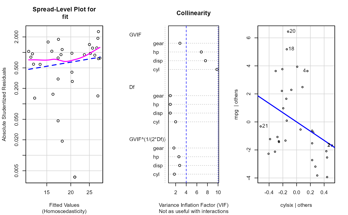
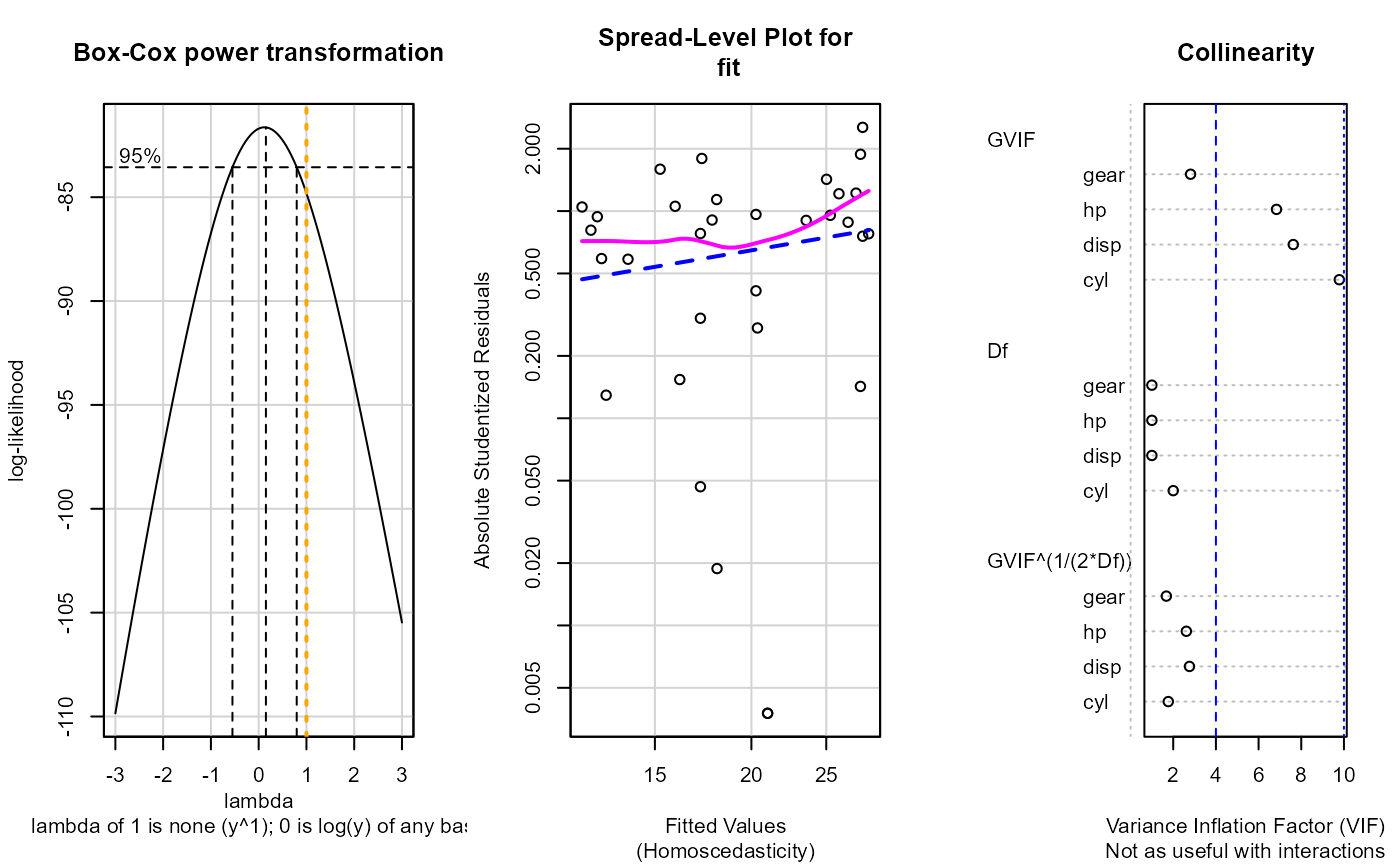
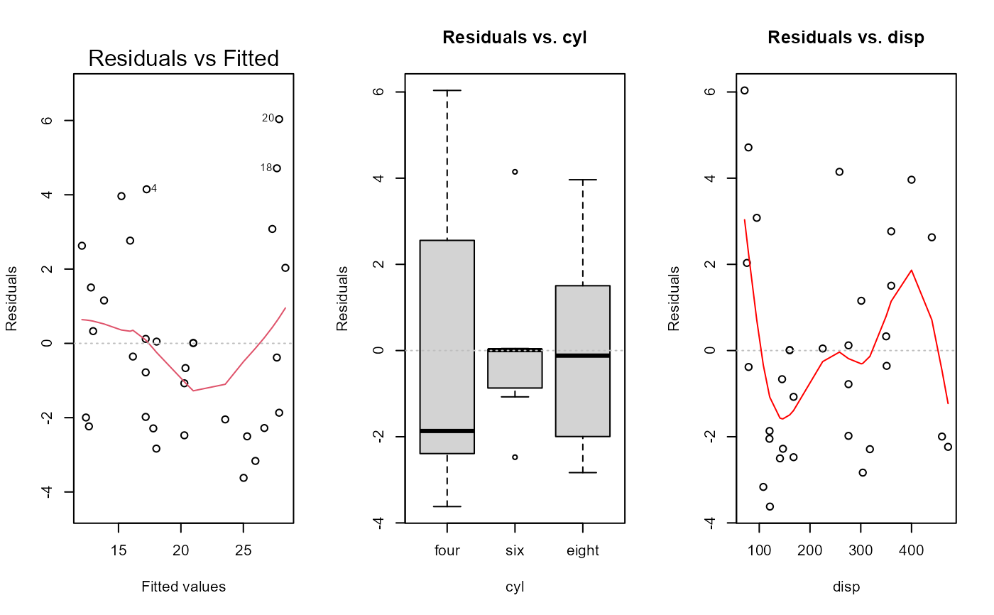
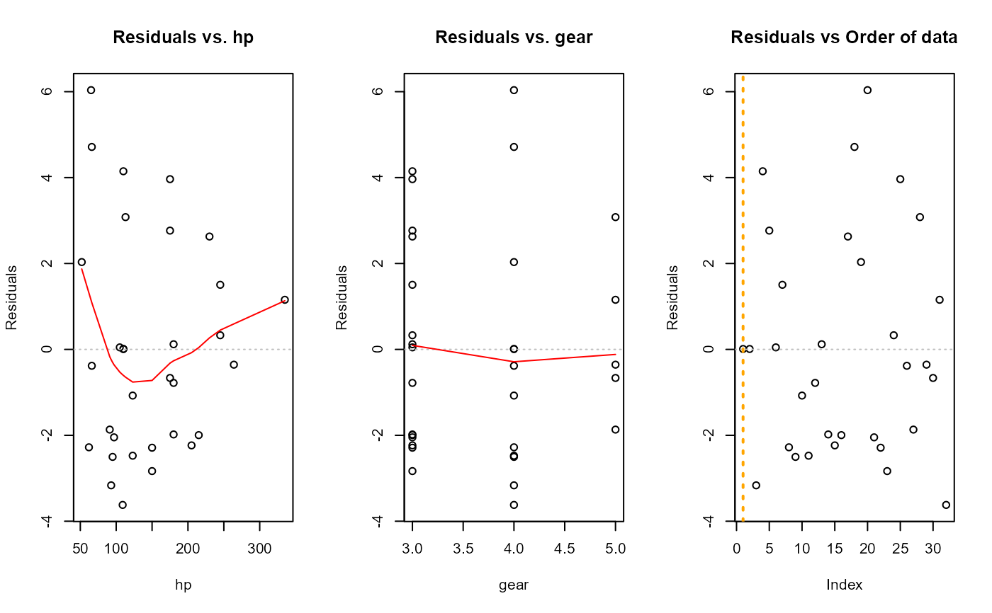
fit <- lm(mpg ~ cyl + disp + hp + gear, data = dat_mtcars_e)
e_plot_lm_diagnostics(fit)



#> Non-constant Variance Score Test 
#> Variance formula: ~ fitted.values 
#> Chisquare = 2.67906, Df = 1, p = 0.10168
#> Warning: Note: Collinearity plot unreliable for predictors that also have interactions in the model.



mod <- stats::formula(mpg ~ cyl + disp + hp + gear)
fit <- lm(mod, data = dat_mtcars_e)
e_plot_lm_diagnostics(fit)



#> Error in stats::model.frame(formula = mod, data = dat_mtcars_e, drop.unused.levels = TRUE) : 
#>   object 'mod' not found
#> Non-constant Variance Score Test 
#> Variance formula: ~ fitted.values 
#> Chisquare = 2.67906, Df = 1, p = 0.10168
#> Warning: Note: Collinearity plot unreliable for predictors that also have interactions in the model.