Multiple regression power analysis
e_lm_power(
  dat = NULL,
  formula_full = NULL,
  formula_red = NULL,
  fit_model_type = c("lm", "lmer")[1],
  n_total,
  n_param_full = NULL,
  n_param_red = NULL,
  sig_level = 0.05,
  weights = NULL,
  sw_print = TRUE,
  sw_plots = TRUE,
  n_plot_ref = NULL
)
Arguments
- dat
observed effect size data set
- formula_full
observed effect size full model formula, used with dat
- formula_red
observed effect size reduced model formula, used with dat
- fit_model_type
"lm" or "lmer", used with dat to specify how formulas should be fit
- n_total
a total sample size value or list of values, used for power curve
- n_param_full
number of parameters in full model, only used if dat is not specified
- n_param_red
number of parameters in reduced model, only used if dat is not specified; must be fewer than n_param_full
- sig_level
Type-I error rate
- weights
observed effect size model fit, if it should be weighted regression
- sw_print
print results
- sw_plots
create histogram and power curve plots
- n_plot_ref
a sample size reference line for the plot; if null, then uses size of data, otherwise uses median of n_total. Histogram is created for first reference value in the list.
Value
list with tables and plots of power analysis results
Examples
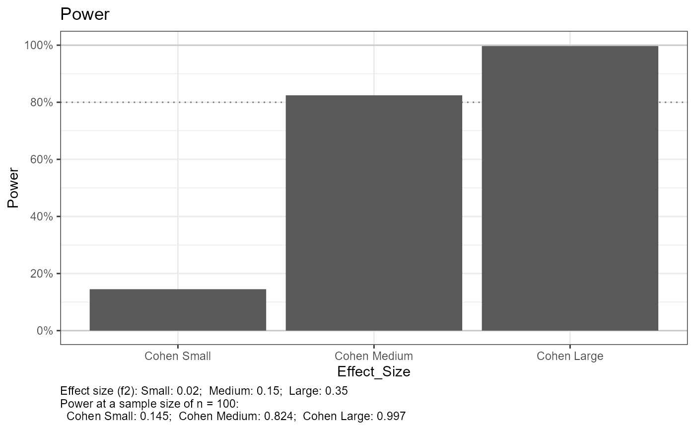
# without data, single n
out <-
e_lm_power(
dat = NULL
, formula_full = NULL
, formula_red = NULL
, n_total = 100
, n_param_full = 10
, n_param_red = 5
, sig_level = 0.05
, weights = NULL
, sw_print = TRUE
, sw_plots = TRUE
, n_plot_ref = NULL
)
#> Setting n_plot_ref = n_total for reference
#> Cohen reference effect size and power =============================
#> Small ---------------
#>
#> Multiple regression power calculation
#>
#> u = 5
#> v = 90
#> f2 = 0.02
#> sig.level = 0.05
#> power = 0.1451294
#>
#> Medium --------------
#>
#> Multiple regression power calculation
#>
#> u = 5
#> v = 90
#> f2 = 0.15
#> sig.level = 0.05
#> power = 0.8244431
#>
#> Large ---------------
#>
#> Multiple regression power calculation
#>
#> u = 5
#> v = 90
#> f2 = 0.35
#> sig.level = 0.05
#> power = 0.997067
#>
#> Joining with `by = join_by(Effect_Size)`
#> e_lm_power, power curve only available when length of n_total > 1
 #> NULL
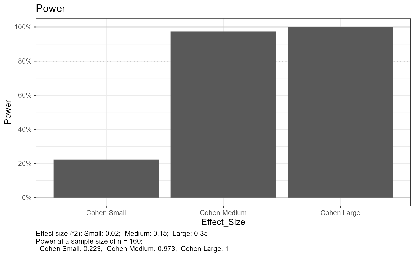
# without data, sequence of n for power curve
out <-
e_lm_power(
dat = NULL
, formula_full = NULL
, formula_red = NULL
, n_total = seq(20, 300, by = 5)
, n_param_full = 10
, n_param_red = 5
, sig_level = 0.05
, weights = NULL
, sw_print = TRUE
, sw_plots = TRUE
, n_plot_ref = NULL
)
#> Setting n_plot_ref = median(n_total) for reference
#> e_lm_power, not printing results when n_total > 1
#> Joining with `by = join_by(Effect_Size)`
#> NULL
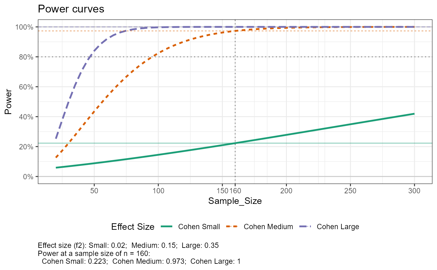
# without data, sequence of n for power curve
out <-
e_lm_power(
dat = NULL
, formula_full = NULL
, formula_red = NULL
, n_total = seq(20, 300, by = 5)
, n_param_full = 10
, n_param_red = 5
, sig_level = 0.05
, weights = NULL
, sw_print = TRUE
, sw_plots = TRUE
, n_plot_ref = NULL
)
#> Setting n_plot_ref = median(n_total) for reference
#> e_lm_power, not printing results when n_total > 1
#> Joining with `by = join_by(Effect_Size)`
 # with data
str(dat_mtcars_e)
#> tibble [32 × 12] (S3: tbl_df/tbl/data.frame)
#> $ model: chr [1:32] "Mazda RX4" "Mazda RX4 Wag" "Datsun 710" "Hornet 4 Drive" ...
#> ..- attr(*, "label")= chr "Model"
#> $ mpg : num [1:32] 21 21 22.8 21.4 18.7 18.1 14.3 24.4 22.8 19.2 ...
#> ..- attr(*, "label")= chr "Miles/(US) gallon"
#> $ cyl : Factor w/ 3 levels "four","six","eight": 2 2 1 2 3 2 3 1 1 2 ...
#> ..- attr(*, "label")= chr "Number of cylinders"
#> $ disp : num [1:32] 160 160 108 258 360 ...
#> ..- attr(*, "label")= chr "Displacement (cu.in.)"
#> $ hp : num [1:32] 110 110 93 110 175 105 245 62 95 123 ...
#> ..- attr(*, "label")= chr "Gross horsepower"
#> $ drat : num [1:32] 3.9 3.9 3.85 3.08 3.15 2.76 3.21 3.69 3.92 3.92 ...
#> ..- attr(*, "label")= chr "Rear axle ratio"
#> $ wt : num [1:32] 2.62 2.88 2.32 3.21 3.44 ...
#> ..- attr(*, "label")= chr "Weight (1000 lbs)"
#> $ qsec : num [1:32] 16.5 17 18.6 19.4 17 ...
#> ..- attr(*, "label")= chr "1/4 mile time"
#> $ vs : Factor w/ 2 levels "V-shaped","straight": 1 1 2 2 1 2 1 2 2 2 ...
#> ..- attr(*, "label")= chr "Engine"
#> $ am : Factor w/ 2 levels "automatic","manual": 2 2 2 1 1 1 1 1 1 1 ...
#> ..- attr(*, "label")= chr "Transmission"
#> $ gear : num [1:32] 4 4 4 3 3 3 3 4 4 4 ...
#> ..- attr(*, "label")= chr "Number of forward gears"
#> $ carb : num [1:32] 4 4 1 1 2 1 4 2 2 4 ...
#> ..- attr(*, "label")= chr "Number of carburetors"
yvar <- "mpg"
xvar_full <- c("cyl", "disp", "hp", "drat", "wt", "qsec")
xvar_red <- c( "hp", "drat", "wt", "qsec")
formula_full <-
stats::as.formula(
paste0(
yvar
, " ~ "
, paste(
xvar_full
, collapse= "+"
)
)
)
formula_red <-
stats::as.formula(
paste0(
yvar
, " ~ "
, paste(
xvar_red
, collapse= "+"
)
)
)
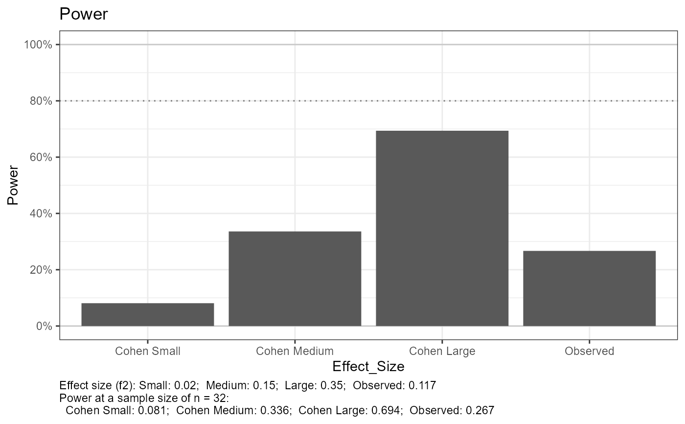
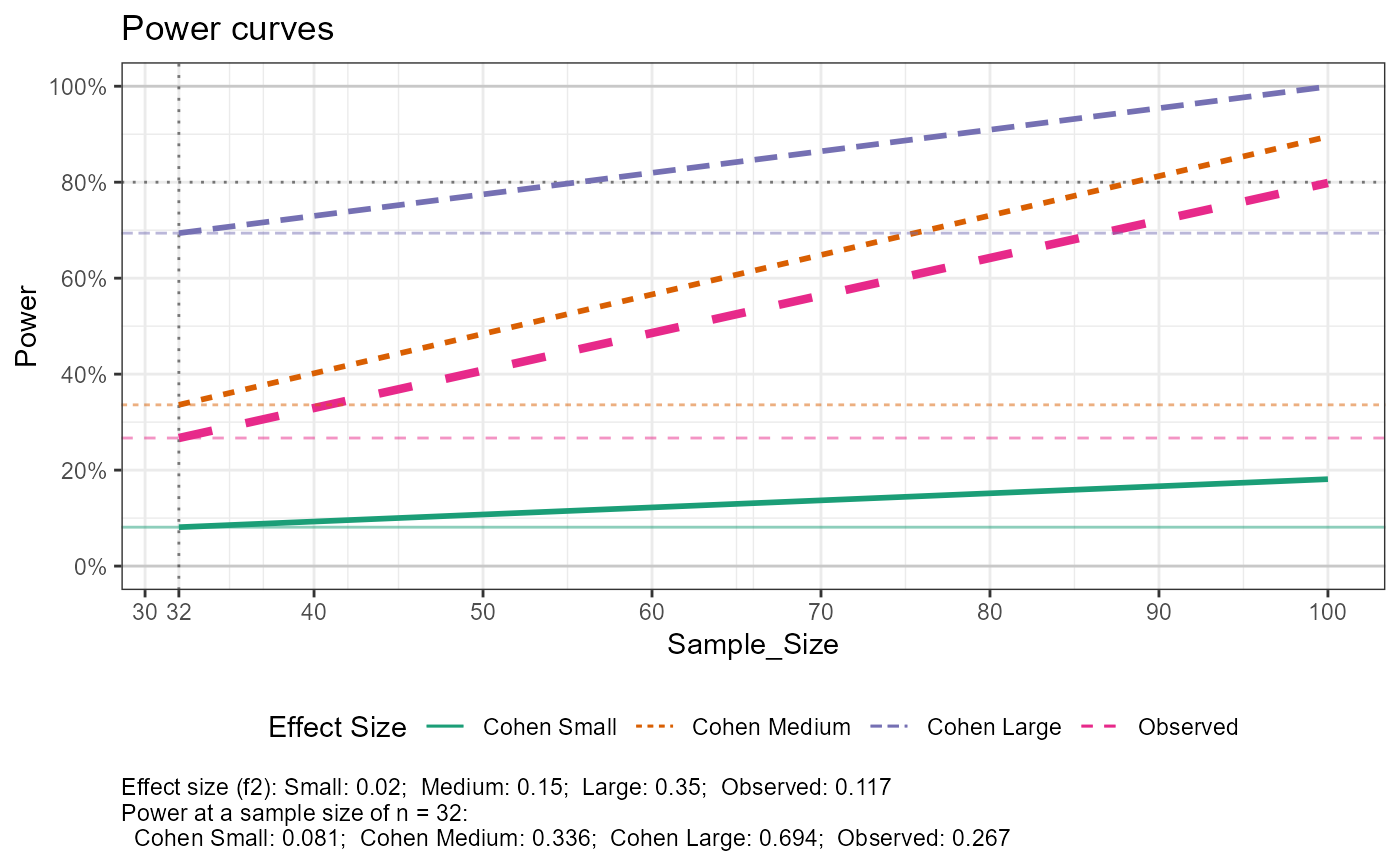
# with data, single n
out <-
e_lm_power(
dat = dat_mtcars_e
, formula_full = formula_full
, formula_red = formula_red
, n_total = 100
, n_param_full = NULL
, n_param_red = NULL
, sig_level = 0.05
, weights = NULL
, sw_print = TRUE
, sw_plots = TRUE
, n_plot_ref = NULL
)
#> Full Model ========================================================
#> mpg ~ cyl + disp + hp + drat + wt + qsec
#> <environment: 0x000001b75809cdb8>
#>
#> Call:
#> lm(formula = formula_full, data = dat)
#>
#> Residuals:
#> Min 1Q Median 3Q Max
#> -4.0821 -1.3663 -0.3597 1.1147 5.1195
#>
#> Coefficients:
#> Estimate Std. Error t value Pr(>|t|)
#> (Intercept) 26.592514 13.093167 2.031 0.0535 .
#> cylsix -2.640596 1.865283 -1.416 0.1697
#> cyleight -2.464875 3.320975 -0.742 0.4652
#> disp 0.006309 0.013588 0.464 0.6466
#> hp -0.022587 0.016043 -1.408 0.1720
#> drat 1.144028 1.483543 0.771 0.4481
#> wt -3.637067 1.354395 -2.685 0.0129 *
#> qsec 0.257633 0.531785 0.484 0.6324
#> ---
#> Signif. codes: 0 '***' 0.001 '**' 0.01 '*' 0.05 '.' 0.1 ' ' 1
#>
#> Residual standard error: 2.549 on 24 degrees of freedom
#> Multiple R-squared: 0.8616, Adjusted R-squared: 0.8212
#> F-statistic: 21.34 on 7 and 24 DF, p-value: 7.409e-09
#>
#> Reduced Model =====================================================
#> mpg ~ hp + drat + wt + qsec
#> <environment: 0x000001b75809cdb8>
#>
#> Call:
#> lm(formula = formula_red, data = dat)
#>
#> Residuals:
#> Min 1Q Median 3Q Max
#> -3.5775 -1.6626 -0.3417 1.1317 5.4422
#>
#> Coefficients:
#> Estimate Std. Error t value Pr(>|t|)
#> (Intercept) 19.25970 10.31545 1.867 0.072785 .
#> hp -0.01784 0.01476 -1.209 0.237319
#> drat 1.65710 1.21697 1.362 0.184561
#> wt -3.70773 0.88227 -4.202 0.000259 ***
#> qsec 0.52754 0.43285 1.219 0.233470
#> ---
#> Signif. codes: 0 '***' 0.001 '**' 0.01 '*' 0.05 '.' 0.1 ' ' 1
#>
#> Residual standard error: 2.539 on 27 degrees of freedom
#> Multiple R-squared: 0.8454, Adjusted R-squared: 0.8225
#> F-statistic: 36.91 on 4 and 27 DF, p-value: 1.408e-10
#>
#> Setting n_plot_ref = the number of observations in the data for reference
#> e_lm_power, not printing results when n_total > 1
#> Joining with `by = join_by(Effect_Size)`
#> e_lm_power, add more values to n_total for a smoother and more accurate curve
# with data
str(dat_mtcars_e)
#> tibble [32 × 12] (S3: tbl_df/tbl/data.frame)
#> $ model: chr [1:32] "Mazda RX4" "Mazda RX4 Wag" "Datsun 710" "Hornet 4 Drive" ...
#> ..- attr(*, "label")= chr "Model"
#> $ mpg : num [1:32] 21 21 22.8 21.4 18.7 18.1 14.3 24.4 22.8 19.2 ...
#> ..- attr(*, "label")= chr "Miles/(US) gallon"
#> $ cyl : Factor w/ 3 levels "four","six","eight": 2 2 1 2 3 2 3 1 1 2 ...
#> ..- attr(*, "label")= chr "Number of cylinders"
#> $ disp : num [1:32] 160 160 108 258 360 ...
#> ..- attr(*, "label")= chr "Displacement (cu.in.)"
#> $ hp : num [1:32] 110 110 93 110 175 105 245 62 95 123 ...
#> ..- attr(*, "label")= chr "Gross horsepower"
#> $ drat : num [1:32] 3.9 3.9 3.85 3.08 3.15 2.76 3.21 3.69 3.92 3.92 ...
#> ..- attr(*, "label")= chr "Rear axle ratio"
#> $ wt : num [1:32] 2.62 2.88 2.32 3.21 3.44 ...
#> ..- attr(*, "label")= chr "Weight (1000 lbs)"
#> $ qsec : num [1:32] 16.5 17 18.6 19.4 17 ...
#> ..- attr(*, "label")= chr "1/4 mile time"
#> $ vs : Factor w/ 2 levels "V-shaped","straight": 1 1 2 2 1 2 1 2 2 2 ...
#> ..- attr(*, "label")= chr "Engine"
#> $ am : Factor w/ 2 levels "automatic","manual": 2 2 2 1 1 1 1 1 1 1 ...
#> ..- attr(*, "label")= chr "Transmission"
#> $ gear : num [1:32] 4 4 4 3 3 3 3 4 4 4 ...
#> ..- attr(*, "label")= chr "Number of forward gears"
#> $ carb : num [1:32] 4 4 1 1 2 1 4 2 2 4 ...
#> ..- attr(*, "label")= chr "Number of carburetors"
yvar <- "mpg"
xvar_full <- c("cyl", "disp", "hp", "drat", "wt", "qsec")
xvar_red <- c( "hp", "drat", "wt", "qsec")
formula_full <-
stats::as.formula(
paste0(
yvar
, " ~ "
, paste(
xvar_full
, collapse= "+"
)
)
)
formula_red <-
stats::as.formula(
paste0(
yvar
, " ~ "
, paste(
xvar_red
, collapse= "+"
)
)
)
# with data, single n
out <-
e_lm_power(
dat = dat_mtcars_e
, formula_full = formula_full
, formula_red = formula_red
, n_total = 100
, n_param_full = NULL
, n_param_red = NULL
, sig_level = 0.05
, weights = NULL
, sw_print = TRUE
, sw_plots = TRUE
, n_plot_ref = NULL
)
#> Full Model ========================================================
#> mpg ~ cyl + disp + hp + drat + wt + qsec
#> <environment: 0x000001b75809cdb8>
#>
#> Call:
#> lm(formula = formula_full, data = dat)
#>
#> Residuals:
#> Min 1Q Median 3Q Max
#> -4.0821 -1.3663 -0.3597 1.1147 5.1195
#>
#> Coefficients:
#> Estimate Std. Error t value Pr(>|t|)
#> (Intercept) 26.592514 13.093167 2.031 0.0535 .
#> cylsix -2.640596 1.865283 -1.416 0.1697
#> cyleight -2.464875 3.320975 -0.742 0.4652
#> disp 0.006309 0.013588 0.464 0.6466
#> hp -0.022587 0.016043 -1.408 0.1720
#> drat 1.144028 1.483543 0.771 0.4481
#> wt -3.637067 1.354395 -2.685 0.0129 *
#> qsec 0.257633 0.531785 0.484 0.6324
#> ---
#> Signif. codes: 0 '***' 0.001 '**' 0.01 '*' 0.05 '.' 0.1 ' ' 1
#>
#> Residual standard error: 2.549 on 24 degrees of freedom
#> Multiple R-squared: 0.8616, Adjusted R-squared: 0.8212
#> F-statistic: 21.34 on 7 and 24 DF, p-value: 7.409e-09
#>
#> Reduced Model =====================================================
#> mpg ~ hp + drat + wt + qsec
#> <environment: 0x000001b75809cdb8>
#>
#> Call:
#> lm(formula = formula_red, data = dat)
#>
#> Residuals:
#> Min 1Q Median 3Q Max
#> -3.5775 -1.6626 -0.3417 1.1317 5.4422
#>
#> Coefficients:
#> Estimate Std. Error t value Pr(>|t|)
#> (Intercept) 19.25970 10.31545 1.867 0.072785 .
#> hp -0.01784 0.01476 -1.209 0.237319
#> drat 1.65710 1.21697 1.362 0.184561
#> wt -3.70773 0.88227 -4.202 0.000259 ***
#> qsec 0.52754 0.43285 1.219 0.233470
#> ---
#> Signif. codes: 0 '***' 0.001 '**' 0.01 '*' 0.05 '.' 0.1 ' ' 1
#>
#> Residual standard error: 2.539 on 27 degrees of freedom
#> Multiple R-squared: 0.8454, Adjusted R-squared: 0.8225
#> F-statistic: 36.91 on 4 and 27 DF, p-value: 1.408e-10
#>
#> Setting n_plot_ref = the number of observations in the data for reference
#> e_lm_power, not printing results when n_total > 1
#> Joining with `by = join_by(Effect_Size)`
#> e_lm_power, add more values to n_total for a smoother and more accurate curve
 # with data, sequence of n for power curve, multiple reference sample sizes
out <-
e_lm_power(
dat = dat_mtcars_e
, formula_full = formula_full
, formula_red = formula_red
, n_total = seq(10, 300, by = 5)
, n_param_full = NULL
, n_param_red = NULL
, sig_level = 0.05
, weights = NULL
, sw_print = TRUE
, sw_plots = TRUE
, n_plot_ref = c(100, 120, 150)
)
#> Full Model ========================================================
#> mpg ~ cyl + disp + hp + drat + wt + qsec
#> <environment: 0x000001b75809cdb8>
#>
#> Call:
#> lm(formula = formula_full, data = dat)
#>
#> Residuals:
#> Min 1Q Median 3Q Max
#> -4.0821 -1.3663 -0.3597 1.1147 5.1195
#>
#> Coefficients:
#> Estimate Std. Error t value Pr(>|t|)
#> (Intercept) 26.592514 13.093167 2.031 0.0535 .
#> cylsix -2.640596 1.865283 -1.416 0.1697
#> cyleight -2.464875 3.320975 -0.742 0.4652
#> disp 0.006309 0.013588 0.464 0.6466
#> hp -0.022587 0.016043 -1.408 0.1720
#> drat 1.144028 1.483543 0.771 0.4481
#> wt -3.637067 1.354395 -2.685 0.0129 *
#> qsec 0.257633 0.531785 0.484 0.6324
#> ---
#> Signif. codes: 0 '***' 0.001 '**' 0.01 '*' 0.05 '.' 0.1 ' ' 1
#>
#> Residual standard error: 2.549 on 24 degrees of freedom
#> Multiple R-squared: 0.8616, Adjusted R-squared: 0.8212
#> F-statistic: 21.34 on 7 and 24 DF, p-value: 7.409e-09
#>
#> Reduced Model =====================================================
#> mpg ~ hp + drat + wt + qsec
#> <environment: 0x000001b75809cdb8>
#>
#> Call:
#> lm(formula = formula_red, data = dat)
#>
#> Residuals:
#> Min 1Q Median 3Q Max
#> -3.5775 -1.6626 -0.3417 1.1317 5.4422
#>
#> Coefficients:
#> Estimate Std. Error t value Pr(>|t|)
#> (Intercept) 19.25970 10.31545 1.867 0.072785 .
#> hp -0.01784 0.01476 -1.209 0.237319
#> drat 1.65710 1.21697 1.362 0.184561
#> wt -3.70773 0.88227 -4.202 0.000259 ***
#> qsec 0.52754 0.43285 1.219 0.233470
#> ---
#> Signif. codes: 0 '***' 0.001 '**' 0.01 '*' 0.05 '.' 0.1 ' ' 1
#>
#> Residual standard error: 2.539 on 27 degrees of freedom
#> Multiple R-squared: 0.8454, Adjusted R-squared: 0.8225
#> F-statistic: 36.91 on 4 and 27 DF, p-value: 1.408e-10
#>
#> e_lm_power, not printing results when n_total > 1
#> Joining with `by = join_by(Effect_Size)`
# with data, sequence of n for power curve, multiple reference sample sizes
out <-
e_lm_power(
dat = dat_mtcars_e
, formula_full = formula_full
, formula_red = formula_red
, n_total = seq(10, 300, by = 5)
, n_param_full = NULL
, n_param_red = NULL
, sig_level = 0.05
, weights = NULL
, sw_print = TRUE
, sw_plots = TRUE
, n_plot_ref = c(100, 120, 150)
)
#> Full Model ========================================================
#> mpg ~ cyl + disp + hp + drat + wt + qsec
#> <environment: 0x000001b75809cdb8>
#>
#> Call:
#> lm(formula = formula_full, data = dat)
#>
#> Residuals:
#> Min 1Q Median 3Q Max
#> -4.0821 -1.3663 -0.3597 1.1147 5.1195
#>
#> Coefficients:
#> Estimate Std. Error t value Pr(>|t|)
#> (Intercept) 26.592514 13.093167 2.031 0.0535 .
#> cylsix -2.640596 1.865283 -1.416 0.1697
#> cyleight -2.464875 3.320975 -0.742 0.4652
#> disp 0.006309 0.013588 0.464 0.6466
#> hp -0.022587 0.016043 -1.408 0.1720
#> drat 1.144028 1.483543 0.771 0.4481
#> wt -3.637067 1.354395 -2.685 0.0129 *
#> qsec 0.257633 0.531785 0.484 0.6324
#> ---
#> Signif. codes: 0 '***' 0.001 '**' 0.01 '*' 0.05 '.' 0.1 ' ' 1
#>
#> Residual standard error: 2.549 on 24 degrees of freedom
#> Multiple R-squared: 0.8616, Adjusted R-squared: 0.8212
#> F-statistic: 21.34 on 7 and 24 DF, p-value: 7.409e-09
#>
#> Reduced Model =====================================================
#> mpg ~ hp + drat + wt + qsec
#> <environment: 0x000001b75809cdb8>
#>
#> Call:
#> lm(formula = formula_red, data = dat)
#>
#> Residuals:
#> Min 1Q Median 3Q Max
#> -3.5775 -1.6626 -0.3417 1.1317 5.4422
#>
#> Coefficients:
#> Estimate Std. Error t value Pr(>|t|)
#> (Intercept) 19.25970 10.31545 1.867 0.072785 .
#> hp -0.01784 0.01476 -1.209 0.237319
#> drat 1.65710 1.21697 1.362 0.184561
#> wt -3.70773 0.88227 -4.202 0.000259 ***
#> qsec 0.52754 0.43285 1.219 0.233470
#> ---
#> Signif. codes: 0 '***' 0.001 '**' 0.01 '*' 0.05 '.' 0.1 ' ' 1
#>
#> Residual standard error: 2.539 on 27 degrees of freedom
#> Multiple R-squared: 0.8454, Adjusted R-squared: 0.8225
#> F-statistic: 36.91 on 4 and 27 DF, p-value: 1.408e-10
#>
#> e_lm_power, not printing results when n_total > 1
#> Joining with `by = join_by(Effect_Size)`
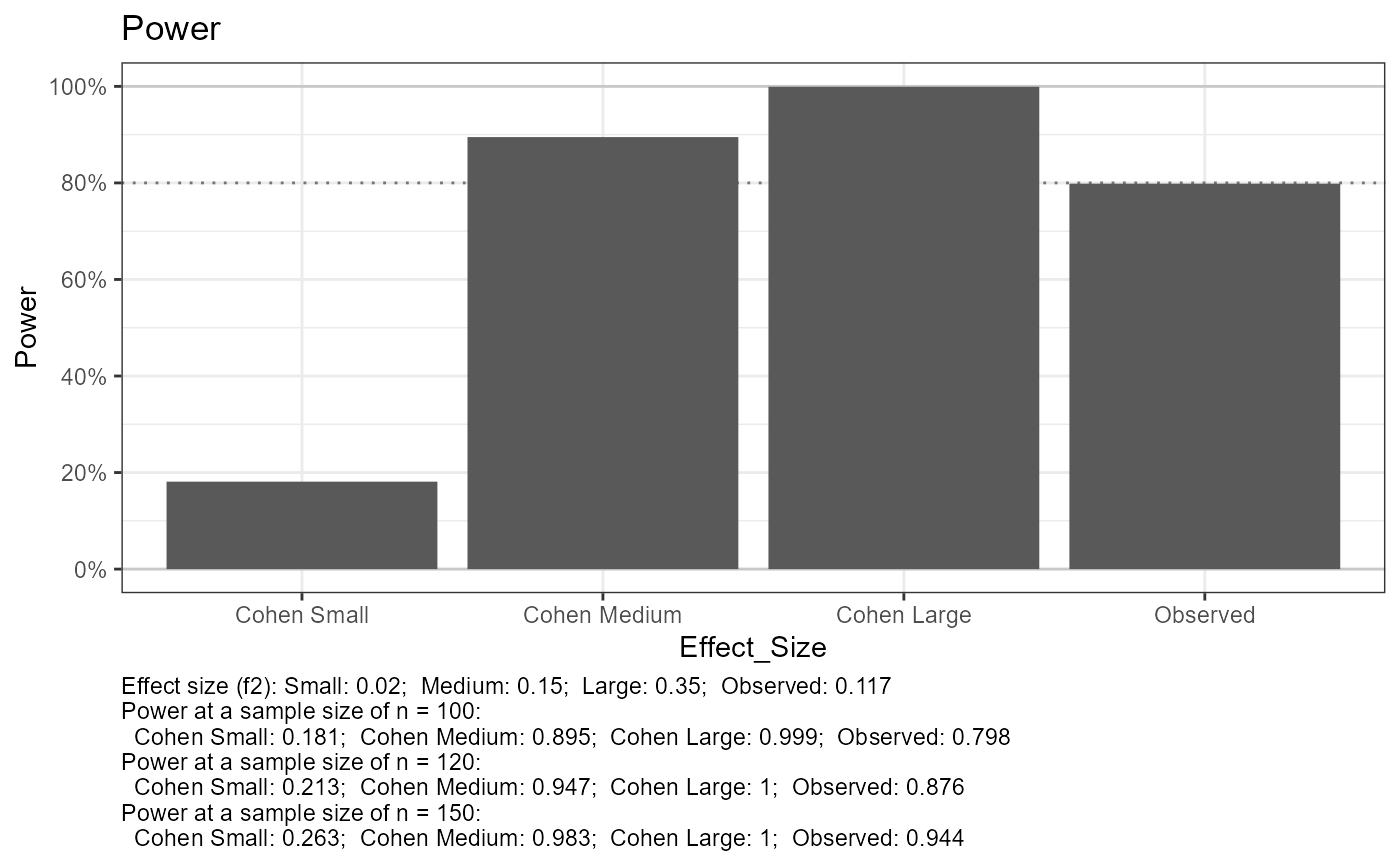
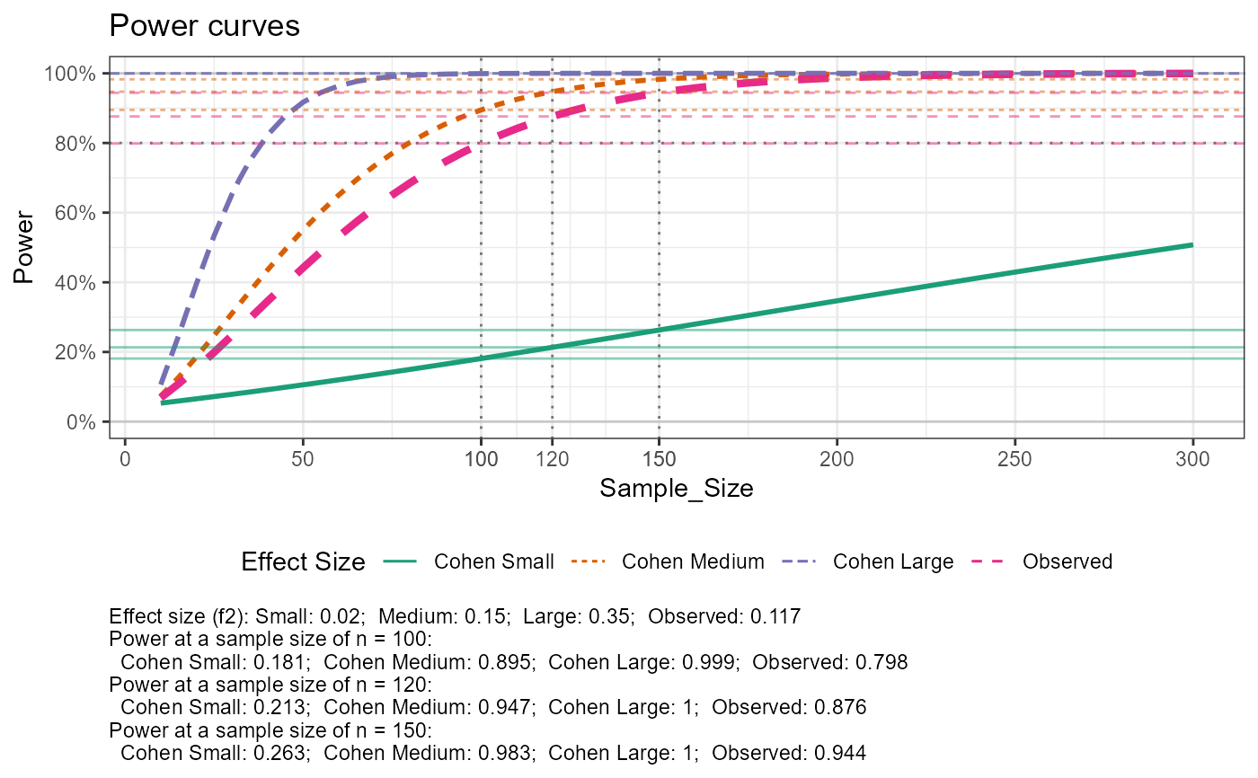 out$tab_power_ref %>% print(width = Inf)
#> # A tibble: 3 × 11
#> n_total n_param_full n_param_red Cohen_small_power Cohen_medium_power
#> <dbl> <dbl> <dbl> <dbl> <dbl>
#> 1 100 7 4 0.181 0.895
#> 2 120 7 4 0.213 0.947
#> 3 150 7 4 0.263 0.983
#> Cohen_large_power obs_power Cohen_small_effect_size Cohen_medium_effect_size
#> <dbl> <dbl> <dbl> <dbl>
#> 1 0.999 0.798 0.02 0.15
#> 2 1.00 0.876 0.02 0.15
#> 3 1.00 0.944 0.02 0.15
#> Cohen_large_effect_size obs_effect_size
#> <dbl> <dbl>
#> 1 0.35 0.117
#> 2 0.35 0.117
#> 3 0.35 0.117
### RMarkdown results reporting
# The results above indicate the following.
#
# 1. With the number of observations
# $n = `r out[["tab_power"]] %>% dplyr::filter(n_total == 100) %>% dplyr::pull(n_total)`$
# and the number of groups
# $k = `r out[["tab_power"]] %>% dplyr::filter(n_total == 100) %>% dplyr::pull(n_groups)`$
# 2. Observed (preliminary) power:
# * `r out[["tab_power"]] %>% dplyr::filter(n_total == 100) %>%
# dplyr::pull(obs_power ) %>% signif(digits = 2)`.
# 3. Cohen small, medium, and large power:
# * `r out[["tab_power"]] %>% dplyr::filter(n_total == 100) %>%
# dplyr::pull(Cohen_small_power ) %>% signif(digits = 2)`,
# * `r out[["tab_power"]] %>% dplyr::filter(n_total == 100) %>%
# dplyr::pull(Cohen_medium_power) %>% signif(digits = 2)`, and
# * `r out[["tab_power"]] %>% dplyr::filter(n_total == 100) %>%
# dplyr::pull(Cohen_large_power ) %>% signif(digits = 2)`.
out$tab_power_ref %>% print(width = Inf)
#> # A tibble: 3 × 11
#> n_total n_param_full n_param_red Cohen_small_power Cohen_medium_power
#> <dbl> <dbl> <dbl> <dbl> <dbl>
#> 1 100 7 4 0.181 0.895
#> 2 120 7 4 0.213 0.947
#> 3 150 7 4 0.263 0.983
#> Cohen_large_power obs_power Cohen_small_effect_size Cohen_medium_effect_size
#> <dbl> <dbl> <dbl> <dbl>
#> 1 0.999 0.798 0.02 0.15
#> 2 1.00 0.876 0.02 0.15
#> 3 1.00 0.944 0.02 0.15
#> Cohen_large_effect_size obs_effect_size
#> <dbl> <dbl>
#> 1 0.35 0.117
#> 2 0.35 0.117
#> 3 0.35 0.117
### RMarkdown results reporting
# The results above indicate the following.
#
# 1. With the number of observations
# $n = `r out[["tab_power"]] %>% dplyr::filter(n_total == 100) %>% dplyr::pull(n_total)`$
# and the number of groups
# $k = `r out[["tab_power"]] %>% dplyr::filter(n_total == 100) %>% dplyr::pull(n_groups)`$
# 2. Observed (preliminary) power:
# * `r out[["tab_power"]] %>% dplyr::filter(n_total == 100) %>%
# dplyr::pull(obs_power ) %>% signif(digits = 2)`.
# 3. Cohen small, medium, and large power:
# * `r out[["tab_power"]] %>% dplyr::filter(n_total == 100) %>%
# dplyr::pull(Cohen_small_power ) %>% signif(digits = 2)`,
# * `r out[["tab_power"]] %>% dplyr::filter(n_total == 100) %>%
# dplyr::pull(Cohen_medium_power) %>% signif(digits = 2)`, and
# * `r out[["tab_power"]] %>% dplyr::filter(n_total == 100) %>%
# dplyr::pull(Cohen_large_power ) %>% signif(digits = 2)`.